Examples / 02

Response surface with four factors and three responses: an API synthesis

A screening has shown four factors of a coupling reaction to be active. The question is no longer whether they act but where they should be set — for three responses at once that do not agree: more temperature and more catalyst bring yield, but also by-product and palladium in the product.

Design: Central composite, rotatable (α = 2)
Runs: 16 + 8 + 6 = 30
Factors: 4, no constraints
Responses: Yield, by-product, residual palladium

The measurements are simulated. They come from three models we set ourselves, plus random scatter — which makes it possible to check at the end whether the analysis finds what is really in there. Every table and chart was computed and drawn by DoEStat.

Step 1 / The question

Four factors, three goals, one compromise

The subject is the last step of an API synthesis, a palladium-catalysed coupling. The four factors are temperature, reaction time, catalyst loading and the equivalents of base. Three quantities are measured on every batch:

Yield in per cent — to be maximised; below 80% the batch is unusable, from 90% the goal is fully met.
By-product in per cent — to be minimised; at most 2.0%, ideally 1.0% or less.
Residual palladium in ppm — to be minimised; at most 30 ppm, ideally 15 ppm or less. This response counts a third as much in the trade-off as the other two, because a downstream purification can still lower it.

Factor	Unit	−α	−1	0	+1	+α
Temperature	°C	60	70	80	90	100
Reaction time	h	1.0	2.0	3.0	4.0	5.0
Catalyst	mol-%	0.50	1.00	1.50	2.00	2.50
Base	eq	1.50	2.00	2.50	3.00	3.50

There are no constraints: every combination of the levels can be run, including the outermost. That is the precondition for a standard design.

Step 2 / Design

A central composite design, and what it promises before the first run

To find an optimum in the interior the model must be able to describe curvature — that is, contain quadratic terms, and for that every factor needs more than two levels. The central composite design provides this at little cost: 16 cube points (all combinations of −1 and +1), 8 axial points (one factor at ±α, the others at the centre) and 6 replicates at the centre. With α = 2 the design is rotatable: the prediction is equally precise at equal distance from the centre in every direction. The axial points lie outside the cube; the ±1 levels are therefore placed so that ±α is still within the safe range.

What the design can do can be checked before a single batch is run:

Term group	Power at 1 σ	Power at 2 σ	VIF
Main effects	99.5	100.0	1.00
Two-factor interactions	96.2	100.0	1.00
Quadratic terms	99.8	100.0	1.05

The variance inflation (VIF) of 1.00 to 1.05 says that the 14 model terms practically do not interfere with one another. An effect the size of one standard deviation is detected with a probability of 96 to over 99%, depending on the term group. The design carries the full quadratic model with 15 degrees of freedom to spare, five of them pure error from the centre runs.

Design and measurements

The runs are listed in the random order in which they were carried out.

Run	Point	Temperature [°C]	Reaction time [h]	Catalyst [mol-%]	Base [eq]	Yield [%]	By-product [%]	Residual palladium [ppm]
1	cube	70	4.0	1.00	2.00	77.1	1.38	16.0
2	cube	70	4.0	2.00	2.00	81.1	1.69	34.0
3	cube	70	2.0	1.00	2.00	69.4	1.13	14.0
4	centre	80	3.0	1.50	2.50	86.8	1.74	23.7
5	cube	90	4.0	2.00	2.00	86.9	3.22	40.0
6	axial	80	3.0	1.50	1.50	78.3	1.94	29.6
7	axial	80	3.0	2.50	2.50	82.2	1.52	50.1
8	axial	60	3.0	1.50	2.50	69.7	1.36	21.8
9	centre	80	3.0	1.50	2.50	84.6	1.46	22.9
10	cube	70	2.0	2.00	2.00	73.4	1.41	36.0
11	axial	80	1.0	1.50	2.50	75.4	0.93	23.4
12	cube	90	4.0	1.00	3.00	79.1	2.51	16.3
13	axial	80	3.0	1.50	3.50	85.3	1.11	19.0
14	centre	80	3.0	1.50	2.50	86.4	1.67	20.3
15	cube	90	2.0	2.00	2.00	83.4	2.03	39.4
16	cube	70	2.0	1.00	3.00	71.0	0.87	13.4
17	axial	80	5.0	1.50	2.50	86.3	2.17	24.1
18	cube	90	2.0	1.00	3.00	77.8	1.50	19.6
19	cube	90	4.0	2.00	3.00	87.7	2.68	31.1
20	centre	80	3.0	1.50	2.50	85.9	1.58	20.6
21	cube	90	2.0	2.00	3.00	87.6	1.53	33.1
22	cube	70	4.0	1.00	3.00	78.5	0.95	13.4
23	axial	80	3.0	0.50	2.50	72.5	1.38	14.4
24	cube	70	2.0	2.00	3.00	75.6	1.12	32.3
25	centre	80	3.0	1.50	2.50	86.9	1.62	24.3
26	cube	90	2.0	1.00	2.00	74.8	1.83	21.0
27	cube	90	4.0	1.00	2.00	78.9	3.04	20.9
28	centre	80	3.0	1.50	2.50	87.3	1.63	23.8
29	axial	100	3.0	1.50	2.50	82.0	3.54	26.8
30	cube	70	4.0	2.00	3.00	83.7	1.19	31.1

Step 3 / Choosing the model

Which order, which terms

First the question of model order. For each response DoEStat compares the linear model, the model with interactions and the quadratic one: does the next order add significantly (sequential p), and does the model then agree with the replicates (lack of fit)? For the yield:

Model order	Sequential p	Lack of fit p	Adj. R²	Pred. R²	Suggested
Linear	< 0.0001	0.0019	0.5703	0.5237
+ interactions	0.7849	0.0012	0.5146	0.4586
+ quadratic terms	< 0.0001	0.4692	0.9701	0.9312	✓

The linear model explains a good half of the variation and shows clear lack of fit. The interactions alone do not help, but the quadratic terms do a great deal: only with them does the lack of fit disappear. For by-product and residual palladium the decision comes out the same way.

Model order for by-product and residual palladium

Model order	Sequential p	Lack of fit p	Adj. R²	Pred. R²	Suggested
Linear	< 0.0001	0.0042	0.7800	0.7079
+ interactions	0.1015	0.0065	0.8259	0.8171
+ quadratic terms	< 0.0001	0.9095	0.9886	0.9805	✓

Model order	Sequential p	Lack of fit p	Adj. R²	Pred. R²	Suggested
Linear	< 0.0001	0.0953	0.8935	0.8685
+ interactions	0.7852	0.0676	0.8797	0.8643
+ quadratic terms	< 0.0001	0.8212	0.9744	0.9516	✓

The full quadratic model has 14 terms. Not every response needs all of them. DoEStat removes backwards whatever is not significant (p-value, α = 0.05) while keeping the hierarchy: a main effect stays as long as a square or an interaction contains it. Every response gets its own model:

Response	Terms in the model	R²	Adj. R²	Pred. R²	Residual s	Lack of fit p	Adequate precision
Yield [%]	10	0.9813	0.9715	0.9437	0.987	0.5177	32.8
By-product [%]	7	0.9886	0.9850	0.9771	0.0827	0.7298	62.5
Residual palladium [ppm]	4	0.9706	0.9659	0.9601	1.65	0.6233	55.6

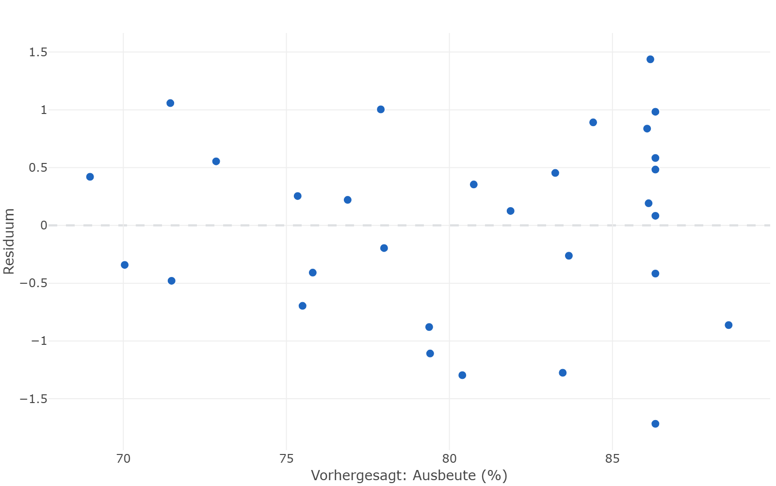
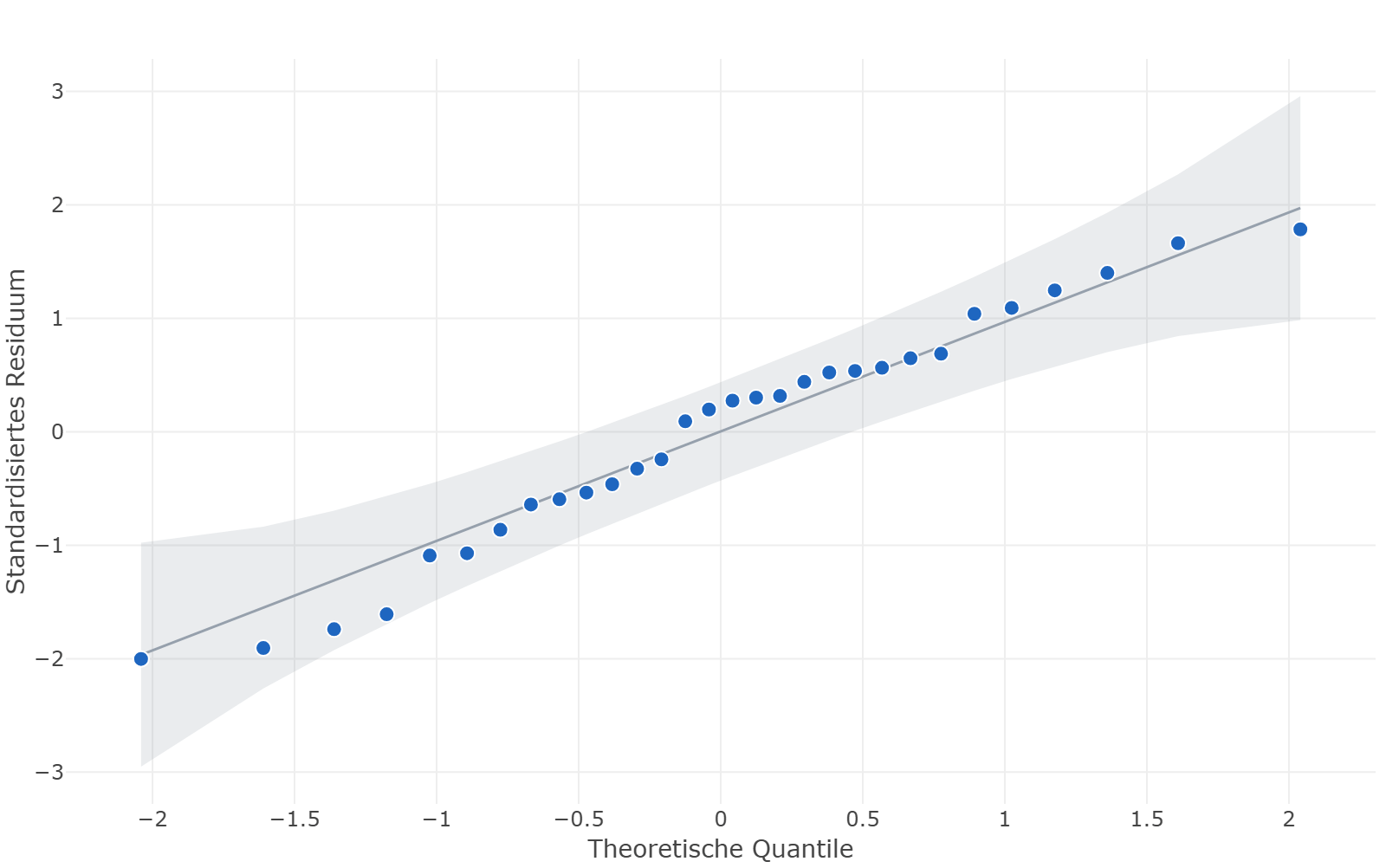
The yield keeps ten terms, the by-product seven, the residual palladium four. For all three the predicted R² is above 0.94 and close to the adjusted one — the models do not just describe the 30 batches, they also predict new ones. The adequate precision, the ratio of signal to noise, is far above the guide value of 4.

Step 4 / Checking the models

Analysis of variance, coefficients, residuals

The analysis of variance of the yield splits the variation: what the model explains, term by term, and what remains — divided into lack of fit and pure error from the six centre runs.

Source	Sum of squares	df	Mean square	F	p
Model	972.4	10	97.24	99.89	< 0.0001
Temperature	210.0	1	210.0	215.77	< 0.0001
Reaction time	159.1	1	159.1	163.47	< 0.0001
Catalyst	217.2	1	217.2	223.12	< 0.0001
Base	37.50	1	37.50	38.52	< 0.0001
Temperature × Reaction time	30.25	1	30.25	31.07	< 0.0001
Temperature × Catalyst	18.49	1	18.49	18.99	0.0003
Temperature²	183.9	1	183.9	188.95	< 0.0001
Reaction time²	49.22	1	49.22	50.56	< 0.0001
Catalyst²	134.5	1	134.5	138.19	< 0.0001
Base²	33.31	1	33.31	34.22	< 0.0001
Residual	18.50	19	0.9735
Lack of fit	13.83	14	0.9877	1.06	0.5177
Pure error	4.668	5	0.9337
Total	990.9	29

The lack of fit is not significant (p = 0.52): what the model does not explain is no larger than the scatter between identical batches. The coefficients in coded units:

Term	Coefficient (coded)	Std. error	t	p	95% CI lower	95% CI upper
Intercept	86.32	0.4028	214.29	< 0.0001	85.47	87.16
Temperature	2.958	0.2014	14.69	< 0.0001	2.537	3.380
Reaction time	2.575	0.2014	12.79	< 0.0001	2.153	2.997
Catalyst	3.008	0.2014	14.94	< 0.0001	2.587	3.430
Base	1.250	0.2014	6.21	< 0.0001	0.8285	1.672
Temperature × Reaction time	−1.375	0.2467	−5.57	< 0.0001	−1.891	−0.8587
Temperature × Catalyst	1.075	0.2467	4.36	0.0003	0.5587	1.591
Temperature²	−2.590	0.1884	−13.75	< 0.0001	−2.984	−2.195
Reaction time²	−1.340	0.1884	−7.11	< 0.0001	−1.734	−0.9453
Catalyst²	−2.215	0.1884	−11.76	< 0.0001	−2.609	−1.820
Base²	−1.102	0.1884	−5.85	< 0.0001	−1.496	−0.7078

All four factors raise the yield, and all four have a negative square: too much of a good thing costs again. The interaction temperature × reaction time is negative — long and hot does harm — and temperature × catalyst is positive.

Analysis of variance and coefficients for by-product and residual palladium

Source	Sum of squares	df	Mean square	F	p
Model	13.05	7	1.864	272.50	< 0.0001
Temperature	6.998	1	6.998	1022.97	< 0.0001
Reaction time	2.483	1	2.483	362.98	< 0.0001
Catalyst	0.1568	1	0.1568	22.92	< 0.0001
Base	1.058	1	1.058	154.71	< 0.0001
Temperature × Reaction time	0.9409	1	0.9409	137.53	< 0.0001
Temperature²	1.311	1	1.311	191.63	< 0.0001
Catalyst²	0.03547	1	0.03547	5.18	0.0329
Residual	0.1505	22	0.006841
Lack of fit	0.1064	17	0.006257	0.71	0.7298
Pure error	0.04413	5	0.008827
Total	13.20	29

Term	Coefficient (coded)	Std. error	t	p	95% CI lower	95% CI upper
Intercept	1.581	0.02388	66.21	< 0.0001	1.531	1.630
Temperature	0.5400	0.01688	31.98	< 0.0001	0.5050	0.5750
Reaction time	0.3217	0.01688	19.05	< 0.0001	0.2867	0.3567
Catalyst	0.08083	0.01688	4.79	< 0.0001	0.04582	0.1158
Base	−0.2100	0.01688	−12.44	< 0.0001	−0.2450	−0.1750
Temperature × Reaction time	0.2425	0.02068	11.73	< 0.0001	0.1996	0.2854
Temperature²	0.2147	0.01551	13.84	< 0.0001	0.1825	0.2469
Catalyst²	−0.03531	0.01551	−2.28	0.0329	−0.06748	−0.003150

Source	Sum of squares	df	Mean square	F	p
Model	2233	4	558.3	206.08	< 0.0001
Temperature	70.73	1	70.73	26.11	< 0.0001
Catalyst	1905	1	1905	703.04	< 0.0001
Base	113.5	1	113.5	41.91	< 0.0001
Catalyst²	144.4	1	144.4	53.29	< 0.0001
Residual	67.73	25	2.709
Lack of fit	52.81	20	2.640	0.88	0.6233
Pure error	14.92	5	2.984
Total	2301	29

Term	Coefficient (coded)	Std. error	t	p	95% CI lower	95% CI upper
Intercept	23.42	0.3880	60.37	< 0.0001	22.62	24.22
Temperature	1.717	0.3360	5.11	< 0.0001	1.025	2.409
Catalyst	8.908	0.3360	26.51	< 0.0001	8.216	9.600
Base	−2.175	0.3360	−6.47	< 0.0001	−2.867	−1.483
Catalyst²	2.239	0.3067	7.30	< 0.0001	1.607	2.871

Residuals of the yield against predicted values: the points scatter evenly around the zero line. — **Residuals against prediction**No structure: the scatter is the same across the whole range of yield.

Normal quantile plot of the standardised residuals of the yield: the points follow the straight line. — **Normality of the residuals**The points follow the line — no transformation of the yield is needed.

Step 5 / Surfaces

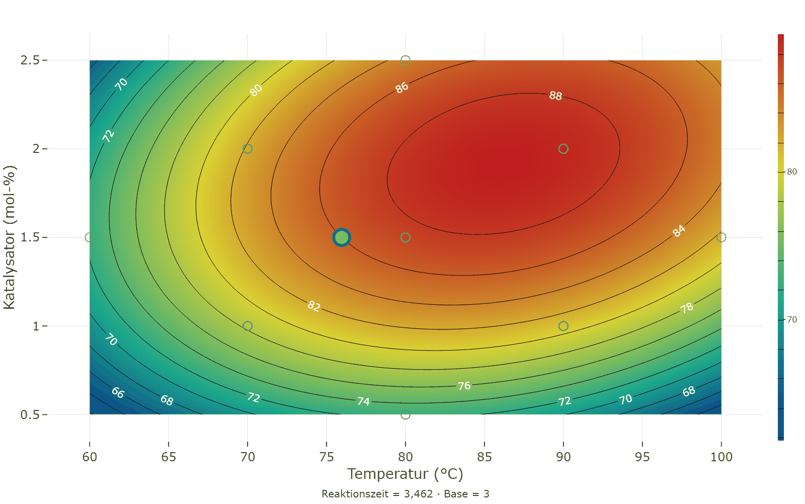
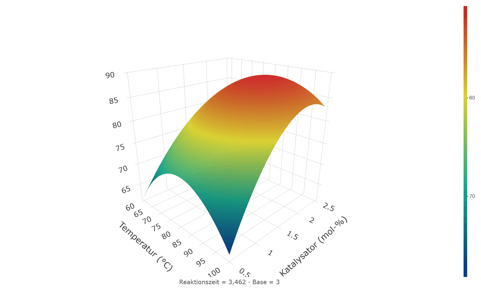
What the models show

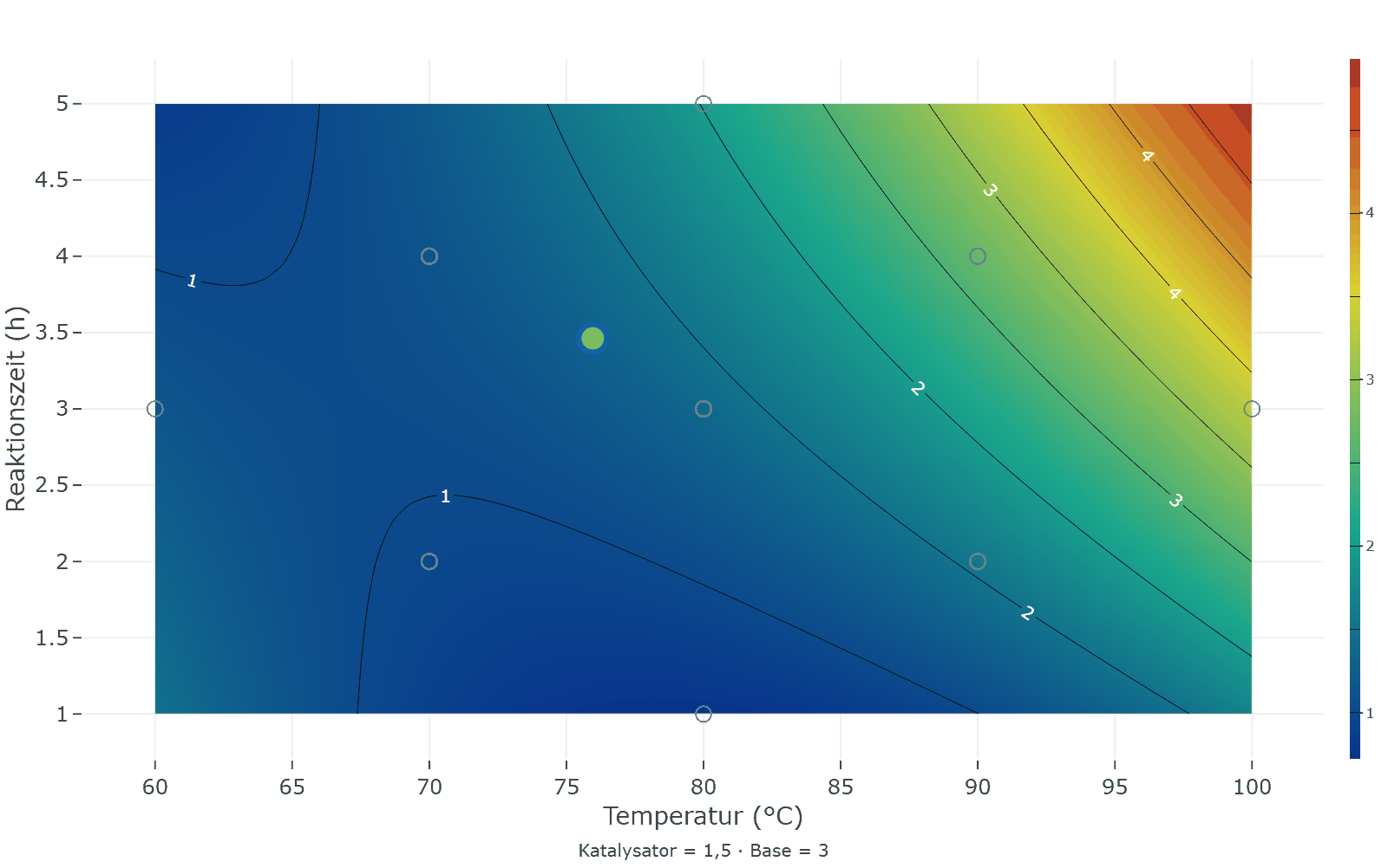
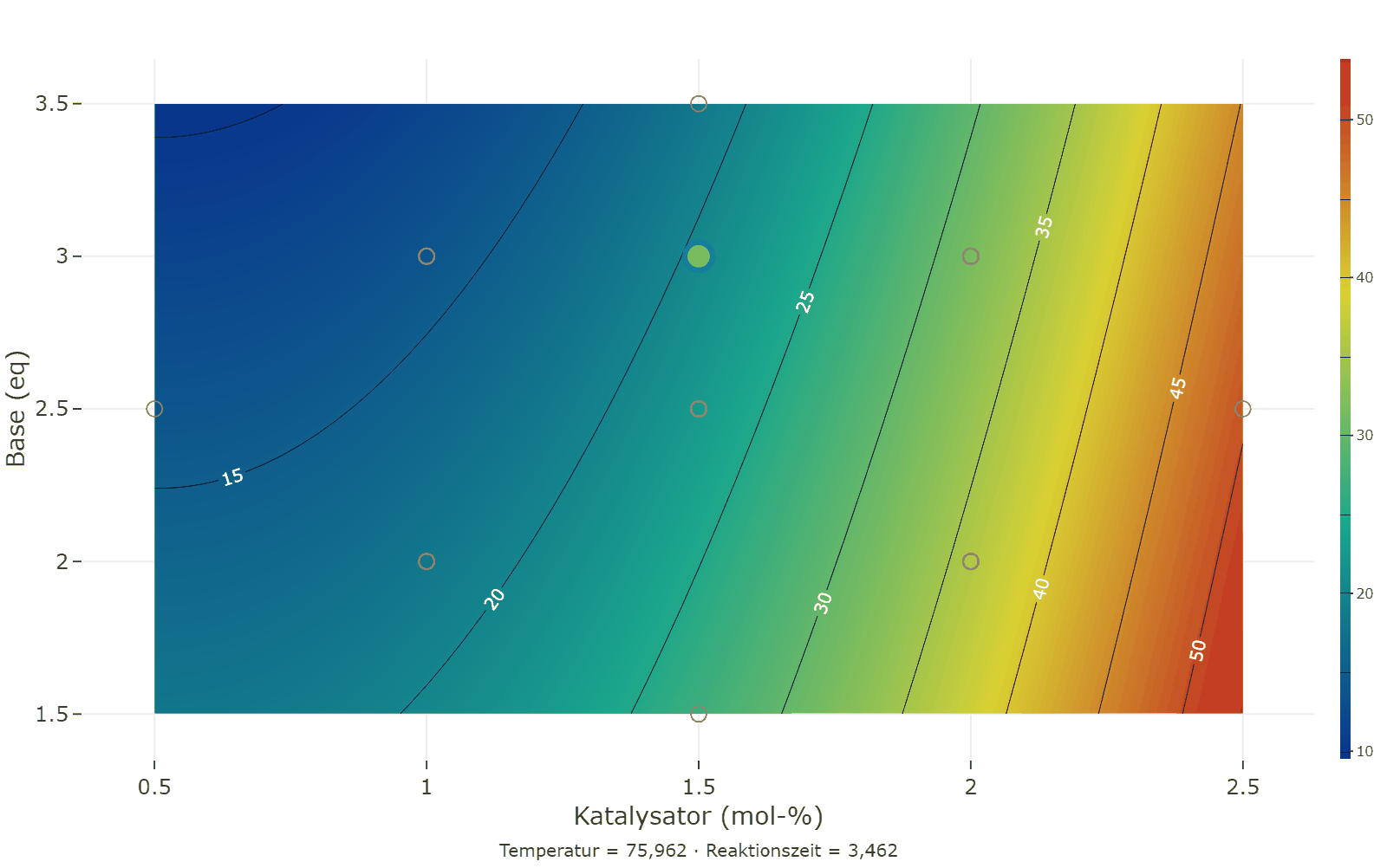
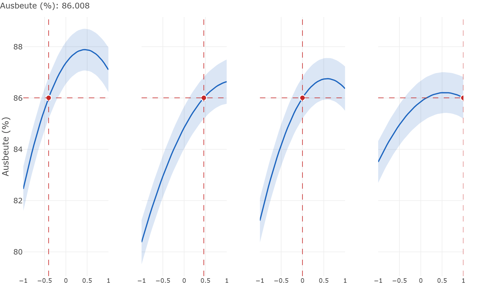
A model with four factors cannot be drawn as one picture. One cuts: two factors on the axes, the other two held at a fixed value — here at that of the optimal setting found later, marked as the point with the blue rim. The grey rings are the runs of the design.

Contour plot of the yield over temperature and catalyst: closed contour lines around a maximum of just over 88 per cent at about 86 degrees and 1.9 mol per cent; the marked optimal setting lies to the lower left of it at 76 degrees and 1.5 mol per cent. — **Yield: temperature × catalyst**The yield alone would peak further up and to the right. The marked compromise lies a good two percentage points below it.

Three-dimensional response surface of the yield over temperature and catalyst: a hill that falls away on all sides. — **The same surface in 3D**A hill: the negative squares of both factors bound it on all sides.

Contour plot of the by-product over temperature and reaction time: the values rise strongly from the lower left to the upper right, the lines are curved. — **By-product: temperature × reaction time**Hot and long drives the by-product — exactly the direction in which the yield at first still rises.

Contour plot of the residual palladium over catalyst and base: the values rise strongly with the catalyst and fall slightly with the base. — **Residual palladium: catalyst × base**Almost only the catalyst determines how much palladium stays in the product; more base lowers it a little.

Prediction profile of the yieldFrom the left: temperature, reaction time, catalyst, base, each in coded units (−1 to +1). For each factor a cut through the surface at the optimal setting, with confidence band. In DoEStat the settings can be moved; all curves follow.

Step 6 / Optimisation

Three goals in one number: desirability

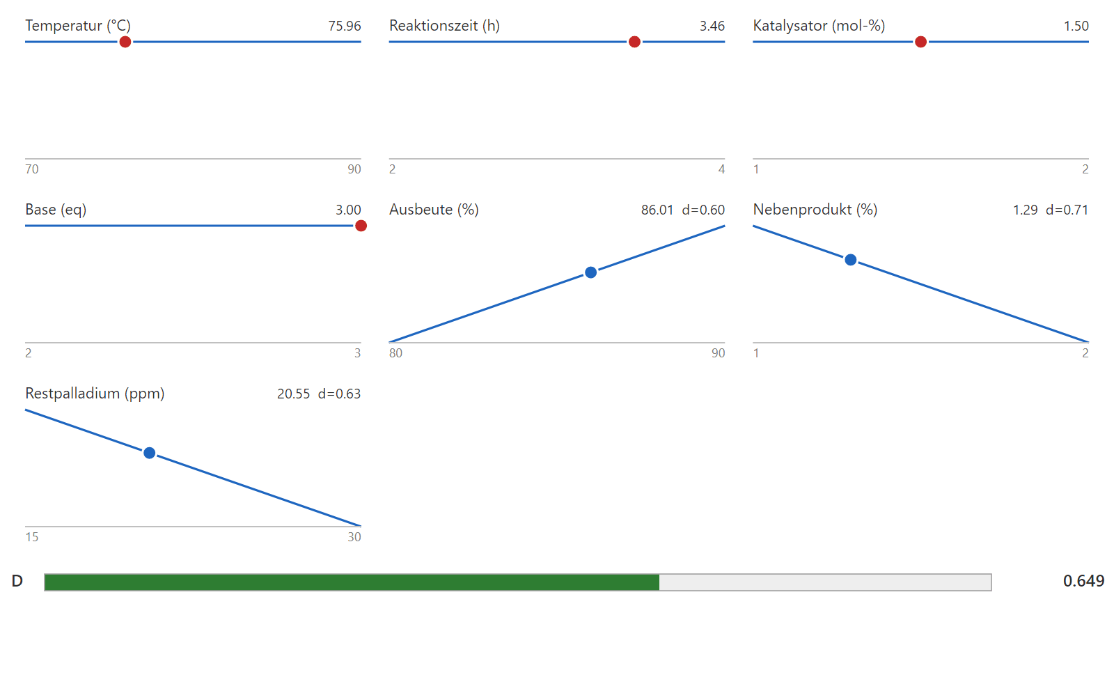
Three surfaces pointing in different directions cannot be overlaid by eye. Desirability turns each response into a number between 0 (specification missed) and 1 (goal fully met) and combines the three into an overall desirability D, weighted by importance. If a single response fails, D is zero — no good value can make up for a bad one. DoEStat searches for the setting with the largest D inside the cube; the axial points have served the model, production is to run in the well-supported core.

Factor	Setting	Unit	coded
Temperature	76.0	°C	−0.40
Reaction time	3.46	h	0.46
Catalyst	1.500	mol-%	0.00
Base	3.000	eq	1.00

Response	Goal	Prediction	95% confidence interval	95% prediction interval	Desirability d	True value
Yield [%]	maximise (80.0 → 90.0)	86.01	85.20 … 86.82	83.79 … 88.23	0.601	85.63
By-product [%]	minimise (2.00 → 1.00)	1.291	1.228 … 1.354	1.109 … 1.474	0.709	1.299
Residual palladium [ppm]	minimise (30.0 → 15.0)	20.55	19.46 … 21.65	16.99 … 24.12	0.630	21.39

The overall desirability is 0.65. The compromise is easy to read: at 76 °C the temperature stays well below the yield maximum, because the by-product would otherwise rise; the catalyst sits at the centre, because more of it carries palladium into the product; the base sits at the upper edge, because it helps all three goals. A second, almost equally good setting (D = 0.64) lies at 74 °C and four hours — colder and longer. DoEStat reports such alternatives; which one to take is for the plant to decide.

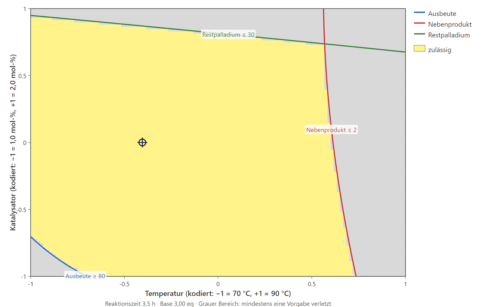
Ramps plot: at the top four sliders for the factors with the optimal setting, below a ramp for each of the three responses with the predicted value as a point, at the bottom a bar for the overall desirability of 0.649. — **Ramps**Each response on its ramp: where the point sits is how far the goal is met.

Overlay plot over temperature and catalyst: a yellow feasible region, bounded on the right by the line by-product equals 2 and at the top by residual palladium equals 30; a crosshair marks the optimal setting in the interior. — **Overlay: the feasible window**Yellow is where all three specifications are met. The setting lies inside the window, clear of its borders.

All responses in one picture

The overlay plot shows only the limits. The overlaid view adds the contour lines of every response in its own colour: one sees not only where the window lies but also how each response behaves inside it. The heavy lines are the limits — solid for a lower limit, dashed for an upper one — the shaded region is the sweet spot, and the dot the optimum. The pictures reach beyond the cube out to the axial points, so that the limits can be seen in full.

Overlaid contour plot over temperature and catalyst: blue contour lines of the yield, red ones of the by-product, green ones of the residual palladium. A shaded region is bounded on the left and at the bottom by the heavy blue line yield equals 80, on the right by the dashed red line by-product equals 2 and at the top by the dashed green line residual palladium equals 30; the optimum lies as a dot in its middle. — **Temperature × catalyst**Three responses, three limits, one window: at the bottom and left yield is missing, on the right there is too much by-product, at the top too much palladium.

Overlaid contour plot over temperature and reaction time: the shaded region lies between the heavy blue line yield equals 80 at the lower left and the dashed red line by-product equals 2 at the upper right; the green lines of the residual palladium run vertically. — **Temperature × reaction time**Hot *and* long exceeds the by-product limit; cold and short does not reach the yield. The palladium does not depend on time at all — its lines are vertical.

Overlaid contour plot over catalyst and base: the shaded region is bounded on the left and at the bottom by the heavy blue line yield equals 80 and on the right by the dashed green line residual palladium equals 30; the optimum lies at 1.5 mol per cent catalyst and 3 equivalents of base. — **Catalyst × base**More catalyst runs into the palladium limit, less into that of the yield. More base pushes both limits apart — which is why it sits at the upper edge.

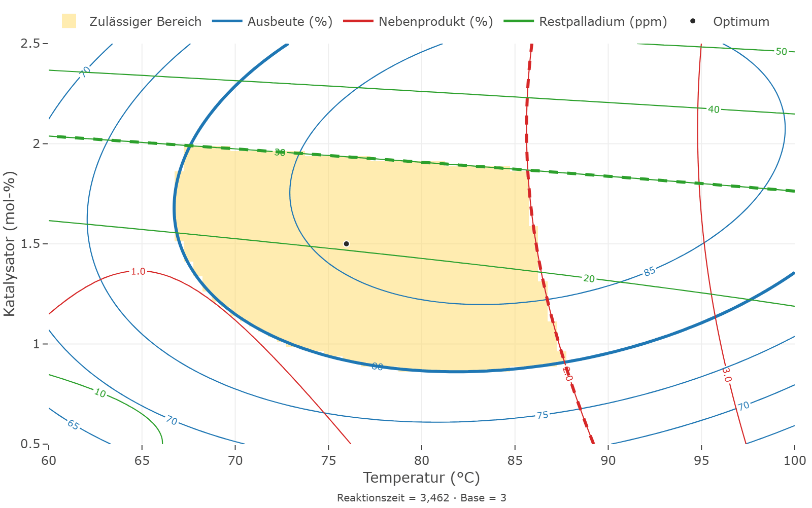
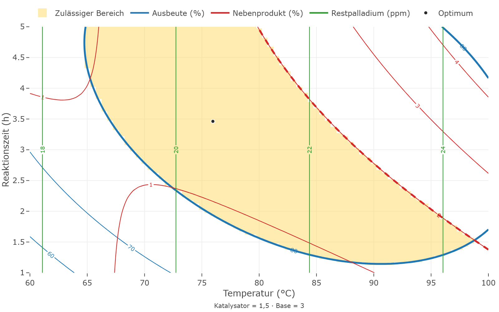
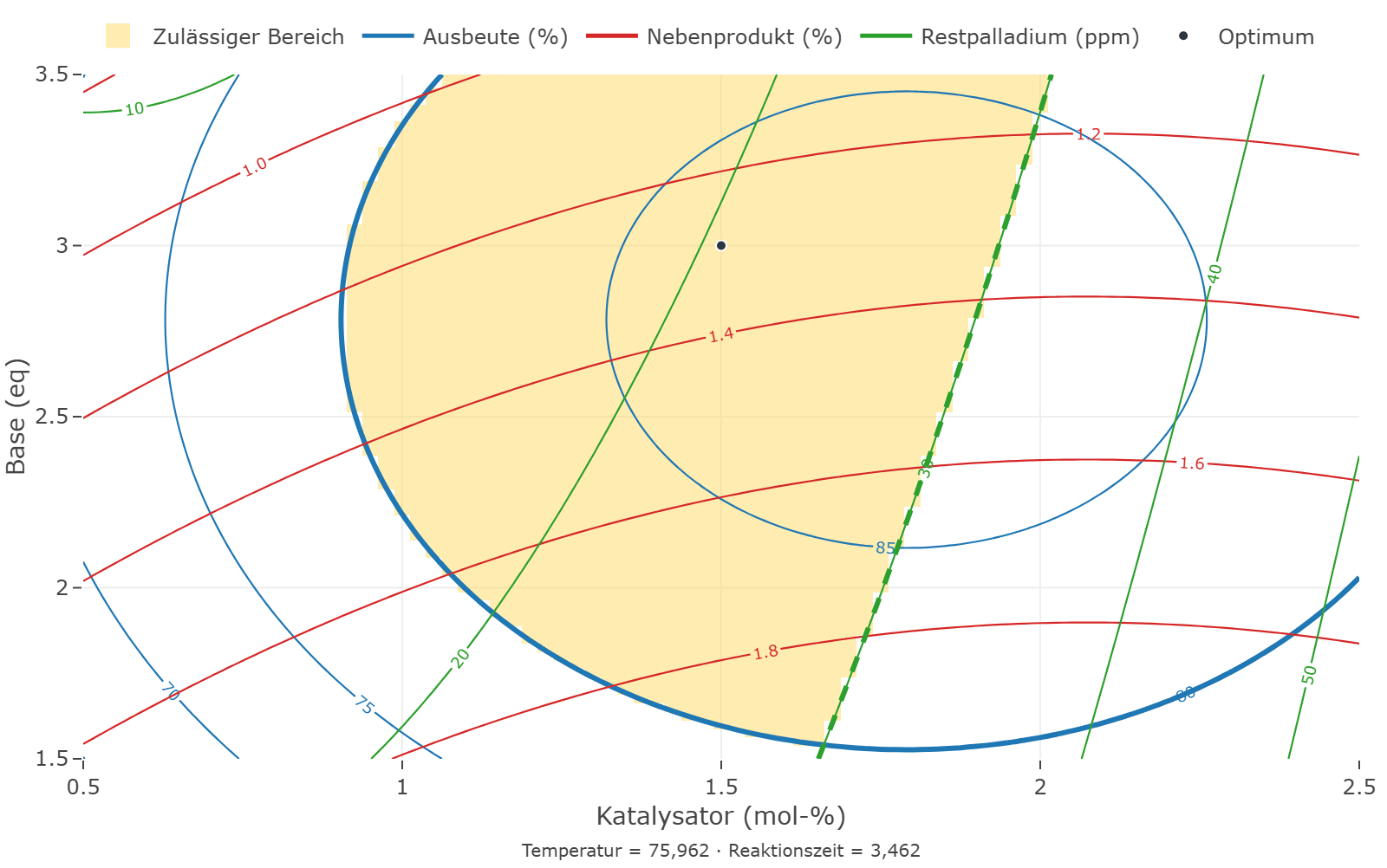
All three cuts pass through the optimum, and in all three it lies clear of the limits. That is the second thing the pictures tell: not only the best setting, but how much latitude it has in every direction.

Step 7 / Confirmation

Three batches at the recommended setting

A prediction is a claim until it has been run. Three confirmation batches at the optimal setting, against the 95% prediction interval for a single batch:

Response	Prediction	95% prediction interval	Confirmation 1	Confirmation 2	Confirmation 3	Joint test p
Yield [%]	86.01	83.79 … 88.23	85.2	85.6	86.8	0.7347
By-product [%]	1.291	1.109 … 1.474	1.19	1.23	1.31	0.6122
Residual palladium [ppm]	20.55	16.99 … 24.12	20.9	22.4	21.6	0.6754

Result: all nine measurements lie within the prediction interval, and no joint test responds. The setting delivers about 86% yield at 1.3% by-product and a little over 20 ppm residual palladium.

Cross-check

What is really in the data

The table sets the true coefficients from which the measurements were simulated beside the estimated ones. A true value of 0 means: in reality this term does not exist.

Response	Term	True	Estimated	95% CI
Yield	Intercept	86.0	86.3	85.5 … 87.2
Yield	Temperature	3.20	2.96	2.54 … 3.38
Yield	Reaction time	2.40	2.57	2.15 … 3.00
Yield	Catalyst	2.90	3.01	2.59 … 3.43
Yield	Base	1.10	1.25	0.828 … 1.67
Yield	Temperature × Reaction time	−1.40	−1.38	−1.89 … −0.859
Yield	Temperature × Catalyst	1.00	1.07	0.559 … 1.59
Yield	Temperature²	−2.60	−2.59	−2.98 … −2.20
Yield	Reaction time²	−1.50	−1.34	−1.73 … −0.945
Yield	Catalyst²	−1.90	−2.21	−2.61 … −1.82
Yield	Base²	−0.800	−1.10	−1.50 … −0.708
By-product	Intercept	1.60	1.58	1.53 … 1.63
By-product	Temperature	0.550	0.540	0.505 … 0.575
By-product	Reaction time	0.300	0.322	0.287 … 0.357
By-product	Catalyst	0.100	0.0808	0.0458 … 0.116
By-product	Base	−0.200	−0.210	−0.245 … −0.175
By-product	Temperature × Reaction time	0.250	0.242	0.200 … 0.285
By-product	Temperature²	0.180	0.215	0.183 … 0.247
By-product	Catalyst²	0	−0.0353	−0.0675 … −0.00315
Residual palladium	Intercept	24.0	23.4	22.6 … 24.2
Residual palladium	Temperature	1.50	1.72	1.02 … 2.41
Residual palladium	Catalyst	9.00	8.91	8.22 … 9.60
Residual palladium	Base	−2.00	−2.17	−2.87 … −1.48
Residual palladium	Catalyst²	2.00	2.24	1.61 … 2.87

For the yield the analysis found exactly the ten terms that exist. Two deviations are instructive. For the by-product a small catalyst square stayed in the model (p = 0.033) that does not exist in truth — with α = 0.05 and three responses with 14 candidates each, one such false hit is to be expected, and at −0.035 it is of no practical consequence. For the residual palladium, conversely, the interaction catalyst × base (truly −1.2 ppm) was lost in the noise. Neither changes anything at the optimal setting: the true values there are in the last column of the optimisation table and all lie within the prediction interval.

Project files

Run it yourself

The example ships with DoEStat: Help ▸ Open sample project ▸ Response surface (RSM) ▸ “Response surface, four factors, three responses: API synthesis”, once with the data only and once with the finished analysis. The same files can be downloaded here.

Project with the datasynthese-wirkflaeche-daten.doejson
Project with the finished analysissynthese-wirkflaeche-auswertung.doejson

Back: screening with ten factors Next: mixture with constraints

Try DoEStat for free

30 days, the full feature set, no payment details. We send the download link by e-mail, usually on the next business day.

Request the trial