
Examples / 03
Mixture with five components and constraints: an emulsion paint
In a formulation no component can be changed without another giving way: the shares add up to 100%. Add bounds and ratio requirements, and what is left of the mixture space is an irregular body for which there is no standard design. This example shows the way from five components and four kinds of constraints to a recipe that meets three responses at once.
- Design
- I-optimal mixture design
- Runs
- 16 + 5 + 4 = 25
- Components
- 5, with bounds, a sum and a ratio constraint
- Responses
- Viscosity, hiding power, wet scrub loss
The measurements are simulated. They come from three models we set ourselves, plus random scatter — which makes it possible to check at the end whether the analysis finds what is really in there. Every table and chart was computed and drawn by DoEStat.
Step 1 / The question
Five components that add up to 100%
The paint consists of binder, pigment, filler, water and an additive package. For each component there is a lower and an upper bound — below the one the paint does not work, above the other it becomes too expensive or can no longer be processed:
| Component | Lower bound [%] | Upper bound [%] | Actually in the design [%] |
|---|---|---|---|
| Binder | 30 | 50 | 30.0 … 50.0 |
| Pigment | 15 | 25 | 15.0 … 25.0 |
| Filler | 5 | 25 | 5.0 … 25.0 |
| Water | 10 | 30 | 10.0 … 30.0 |
| Additive | 2 | 6 | 2.0 … 6.0 |
In addition there are two conditions that link several components:
- Pigment + filler ≤ 40% — the dispersion no longer binds more solids reliably.
- Binder : pigment ≥ 1.6 — every part of pigment needs at least 1.6 parts of binder.
Three quantities are measured: the viscosity in Krebs units (target 100 KU, 90 to 110 allowed), the hiding power as contrast ratio (to be maximised, at least 96%, ideally 98%) and the wet scrub loss in micrometres (to be minimised, at most 20 µm, ideally 8 µm). The wet scrub loss counts somewhat less in the trade-off than the other two.
Step 2 / The region
What the constraints leave of the mixture space
Five shares adding up to one span a four-dimensional body. Without bounds it would be a regular simplex, and the classical simplex designs would fit. The lower and upper bounds cut a body with 24 vertices out of it; the sum and the ratio constraint cut once more and leave 28 vertices. DoEStat computes this body from the constraints as entered — the ratio constraint is written as what it is, a straight line: binder − 1.6 · pigment ≥ 0.
The vertices, the midpoints of edges and faces and the centroid give 124 candidate points. Running all of them would be a waste: a quadratic mixture model for five components has 15 coefficients.
Step 3 / Design
16 points for the model, 9 for the check
An optimal design selects from the candidates the points with which the desired model can be estimated best. The I-criterion is chosen: it minimises the average prediction variance over the whole feasible region — the right thing when a recipe is to be predicted at the end. 16 points carry the model; added to these are five points that DoEStat places in the gaps to expose lack of fit, and four replicates for pure error.
| Run | Point | Binder [%] | Pigment [%] | Filler [%] | Water [%] | Additive [%] | Viscosity [KU] | Hiding power [%] | Wet scrub loss [µm] |
|---|---|---|---|---|---|---|---|---|---|
| 1 | vertex | 44.0 | 15.0 | 25.0 | 10.0 | 6.0 | 157.1 | 95.25 | 15.7 |
| 2 | lack-of-fit | 43.9 | 24.4 | 6.5 | 19.6 | 5.6 | 98.6 | 96.75 | 9.3 |
| 3 | vertex | 50.0 | 15.0 | 23.0 | 10.0 | 2.0 | 100.1 | 95.20 | 12.1 |
| 4 | edge midpoint | 50.0 | 15.0 | 12.0 | 17.0 | 6.0 | 115.0 | 94.07 | 4.4 |
| 5 | lack-of-fit | 36.6 | 16.6 | 20.4 | 23.9 | 2.5 | 60.7 | 94.90 | 21.3 |
| 6 | replicate | 41.1 | 19.7 | 14.0 | 21.1 | 4.0 | 83.8 | 95.97 | 13.4 |
| 7 | replicate | 50.0 | 20.0 | 16.0 | 10.0 | 4.0 | 128.5 | 96.76 | 6.4 |
| 8 | face centroid | 50.0 | 20.0 | 16.0 | 10.0 | 4.0 | 135.2 | 97.04 | 8.2 |
| 9 | lack-of-fit | 46.0 | 15.4 | 11.1 | 25.1 | 2.4 | 38.8 | 93.52 | 8.1 |
| 10 | edge midpoint | 44.0 | 25.0 | 15.0 | 14.0 | 2.0 | 96.9 | 97.33 | 13.8 |
| 11 | lack-of-fit | 33.7 | 20.2 | 14.3 | 26.6 | 5.1 | 72.3 | 96.27 | 21.5 |
| 12 | edge midpoint | 39.0 | 15.0 | 14.0 | 30.0 | 2.0 | 27.8 | 93.57 | 15.7 |
| 13 | face centroid | 38.8 | 24.2 | 5.0 | 28.0 | 4.0 | 45.7 | 95.72 | 16.1 |
| 14 | replicate | 38.8 | 24.2 | 5.0 | 28.0 | 4.0 | 49.5 | 96.29 | 16.6 |
| 15 | vertex | 50.0 | 25.0 | 5.0 | 14.0 | 6.0 | 128.7 | 96.96 | 6.8 |
| 16 | edge midpoint | 46.0 | 15.0 | 5.0 | 30.0 | 4.0 | 32.0 | 92.86 | 8.8 |
| 17 | centroid | 41.1 | 19.7 | 14.0 | 21.1 | 4.0 | 81.1 | 96.25 | 13.2 |
| 18 | lack-of-fit | 45.0 | 15.9 | 19.6 | 16.3 | 3.2 | 88.5 | 95.51 | 12.5 |
| 19 | edge midpoint | 40.2 | 18.8 | 5.0 | 30.0 | 6.0 | 49.8 | 94.42 | 13.1 |
| 20 | face centroid | 38.0 | 15.0 | 25.0 | 18.0 | 4.0 | 95.6 | 94.88 | 19.7 |
| 21 | edge midpoint | 50.0 | 20.0 | 5.0 | 23.0 | 2.0 | 44.8 | 95.04 | 6.4 |
| 22 | edge midpoint | 35.0 | 21.9 | 18.1 | 19.0 | 6.0 | 126.3 | 97.40 | 17.4 |
| 23 | vertex | 30.0 | 15.0 | 19.0 | 30.0 | 6.0 | 61.1 | 94.58 | 22.9 |
| 24 | replicate | 41.1 | 19.7 | 14.0 | 21.1 | 4.0 | 82.8 | 96.42 | 12.5 |
| 25 | vertex | 30.0 | 18.7 | 21.3 | 28.0 | 2.0 | 44.1 | 95.77 | 25.0 |
Among the 16 model points are five vertices, seven edge midpoints, three face centroids and the centroid. The last column of the bounds table above shows that the design moves every component across its whole allowed range — as far as the two linking constraints permit.
Step 4 / Models
Scheffé models: linear, and with blending terms where needed
Mixture models have no constant — it is contained in the linear terms, because the shares add up to one. The linear terms describe how each component acts on its own; the blending terms (products of two components) describe where two components together do more or less than the sum.
| Response | Model order | Sequential p | Lack of fit p | Adj. R² | Pred. R² |
|---|---|---|---|---|---|
| Viscosity | Linear | < 0.0001 | 0.1250 | 0.9816 | 0.9742 |
| Viscosity | Quadratic | 0.0102 | 0.5310 | 0.9937 | 0.9445 |
| Hiding power | Linear | < 0.0001 | 0.2796 | 0.9151 | 0.8922 |
| Hiding power | Quadratic | 0.0296 | 0.7215 | 0.9625 | 0.8580 |
| Wet scrub loss | Linear | < 0.0001 | 0.0621 | 0.9247 | 0.9006 |
| Wet scrub loss | Quadratic | 0.1797 | 0.0853 | 0.9466 | 0.3392 |
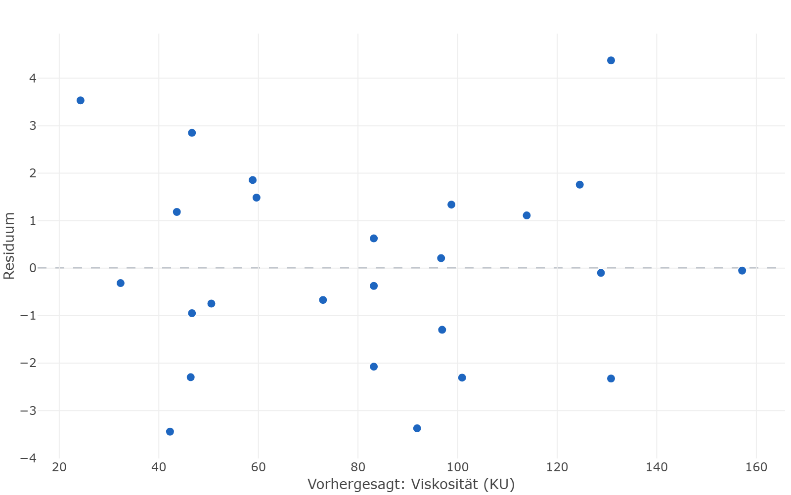
The table is a warning. For all three responses the full quadratic model has the higher adjusted R² — but the lower predicted one, for the wet scrub loss as low as 0.34. Ten blending terms on 25 runs are too many: the model follows the noise. The answer lies in between. DoEStat starts from the quadratic model, works backwards and keeps only the blending terms that are significant; the linear terms always stay.
| Response | Blending terms in the model | R² | Adj. R² | Pred. R² | Residual s | Lack of fit p |
|---|---|---|---|---|---|---|
| Viscosity [KU] | 2 | 0.9968 | 0.9957 | 0.9941 | 2.37 | 0.8019 |
| Hiding power [%] | 4 | 0.9722 | 0.9583 | 0.9161 | 0.255 | 0.6573 |
| Wet scrub loss [µm] | 2 | 0.9684 | 0.9578 | 0.9317 | 1.15 | 0.1630 |
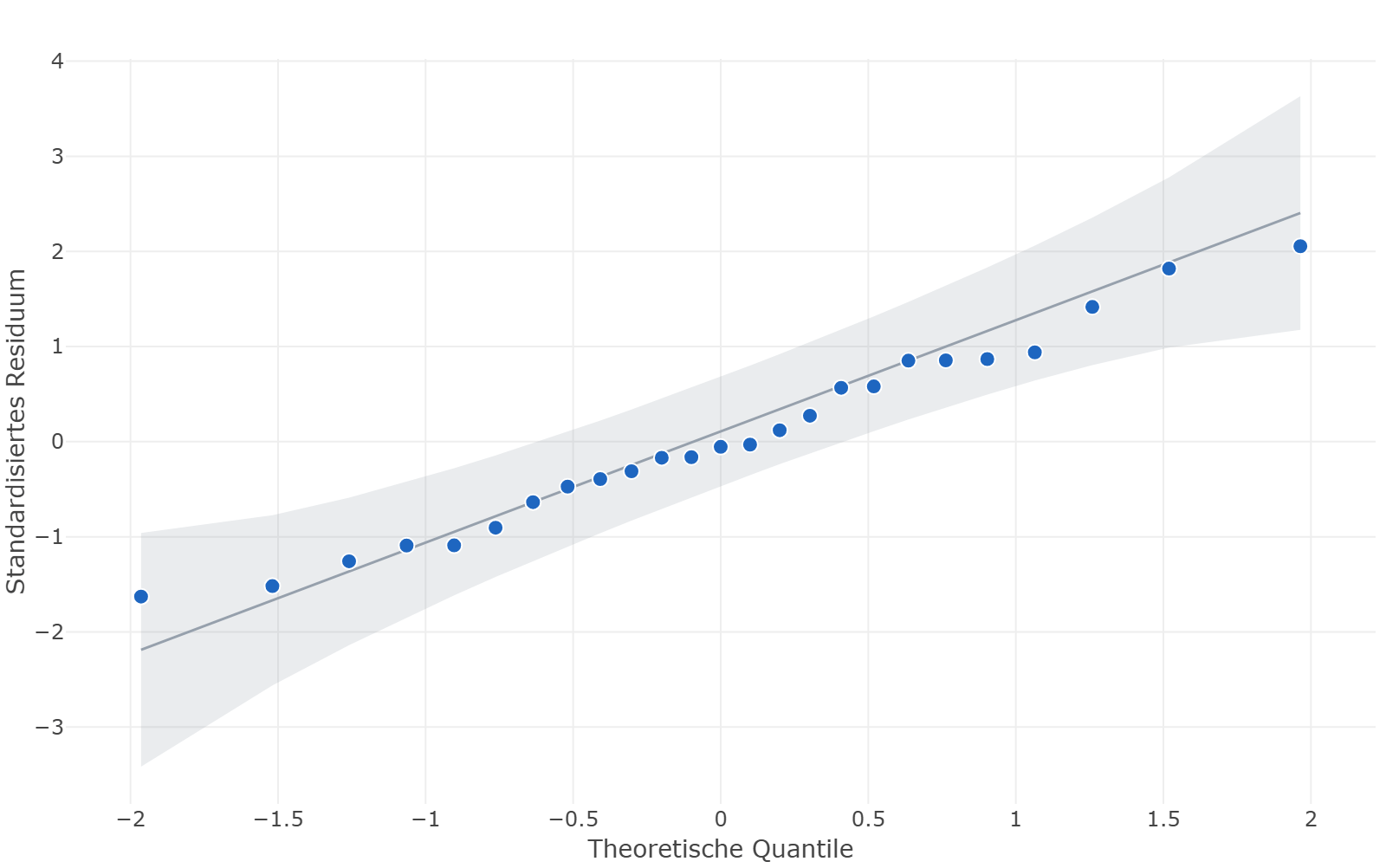
Two to four blending terms per response are enough. The predicted R² is now above 0.91 for all three, and the lack of fit is nowhere significant.
| Term (pseudo-components) | Viscosity [KU] | Hiding power [%] | Wet scrub loss [µm] |
|---|---|---|---|
| Binder | 83.7 | 93.4 | −11.7 |
| Pigment | 110 | 80.9 | 33.5 |
| Filler | 116 | 96.9 | 37.4 |
| Water | −43.5 | 92.1 | 23.6 |
| Additive | 622 | 95.9 | 0.675 |
| Binder × Pigment | · | 33.7 | · |
| Pigment × Filler | 161 | 34.5 | −49.1 |
| Pigment × Water | · | 31.4 | · |
| Pigment × Additive | · | 44.8 | · |
| Filler × Water | · | · | −17.8 |
| Water × Additive | −461 | · | · |
The coefficients are in pseudo-components: every component is rescaled so that 0 is its lower bound. A linear coefficient is then the predicted response at a corner of the feasible region — a recipe one could actually mix. In real shares it would be the prediction for “100% additive”, a number without meaning. The predictions themselves are the same in both notations.
Analyses of variance of the three models
In the analysis of variance of a mixture the linear terms appear as one line: asking whether a single linear coefficient is zero would be asking whether the pure component has a response of zero. The sensible question is whether the response depends on the recipe at all.
| Source | Sum of squares | df | Mean square | F | p |
|---|---|---|---|---|---|
| Model | 31340 | 6 | 5223 | 933.39 | < 0.0001 |
| Linear mixture | 30959 | 4 | 7740 | 1383.07 | < 0.0001 |
| Pigment × Filler | 138.6 | 1 | 138.6 | 24.77 | < 0.0001 |
| Water × Additive | 275.2 | 1 | 275.2 | 49.18 | < 0.0001 |
| Residual | 100.7 | 18 | 5.596 | ||
| Lack of fit | 67.34 | 14 | 4.810 | 0.58 | 0.8019 |
| Pure error | 33.39 | 4 | 8.348 | ||
| Total | 31440 | 24 |
| Source | Sum of squares | df | Mean square | F | p |
|---|---|---|---|---|---|
| Model | 36.26 | 8 | 4.533 | 69.88 | < 0.0001 |
| Linear mixture | 34.66 | 4 | 8.666 | 133.60 | < 0.0001 |
| Binder × Pigment | 0.8287 | 1 | 0.8287 | 12.78 | 0.0025 |
| Pigment × Filler | 1.513 | 1 | 1.513 | 23.32 | 0.0002 |
| Pigment × Water | 0.9211 | 1 | 0.9211 | 14.20 | 0.0017 |
| Pigment × Additive | 0.5558 | 1 | 0.5558 | 8.57 | 0.0099 |
| Residual | 1.038 | 16 | 0.06486 | ||
| Lack of fit | 0.7329 | 12 | 0.06107 | 0.80 | 0.6573 |
| Pure error | 0.3049 | 4 | 0.07623 | ||
| Total | 37.30 | 24 |
| Source | Sum of squares | df | Mean square | F | p |
|---|---|---|---|---|---|
| Model | 730.6 | 6 | 121.8 | 91.86 | < 0.0001 |
| Linear mixture | 707.2 | 4 | 176.8 | 133.36 | < 0.0001 |
| Pigment × Filler | 12.50 | 1 | 12.50 | 9.43 | 0.0066 |
| Filler × Water | 6.280 | 1 | 6.280 | 4.74 | 0.0431 |
| Residual | 23.86 | 18 | 1.326 | ||
| Lack of fit | 21.67 | 14 | 1.548 | 2.83 | 0.1630 |
| Pure error | 2.192 | 4 | 0.5479 | ||
| Total | 754.5 | 24 |
Step 5 / Component effects
Which component moves which response
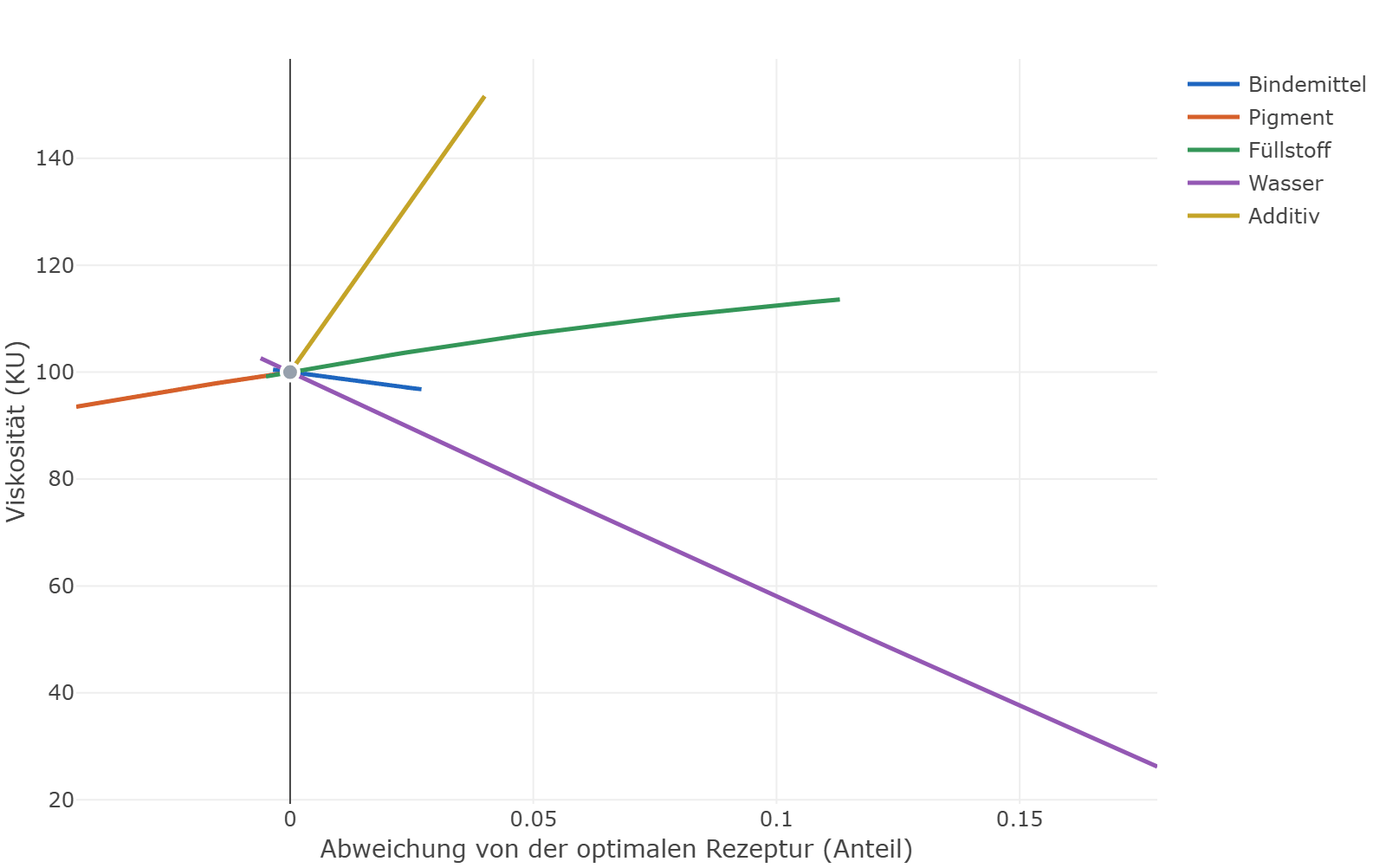
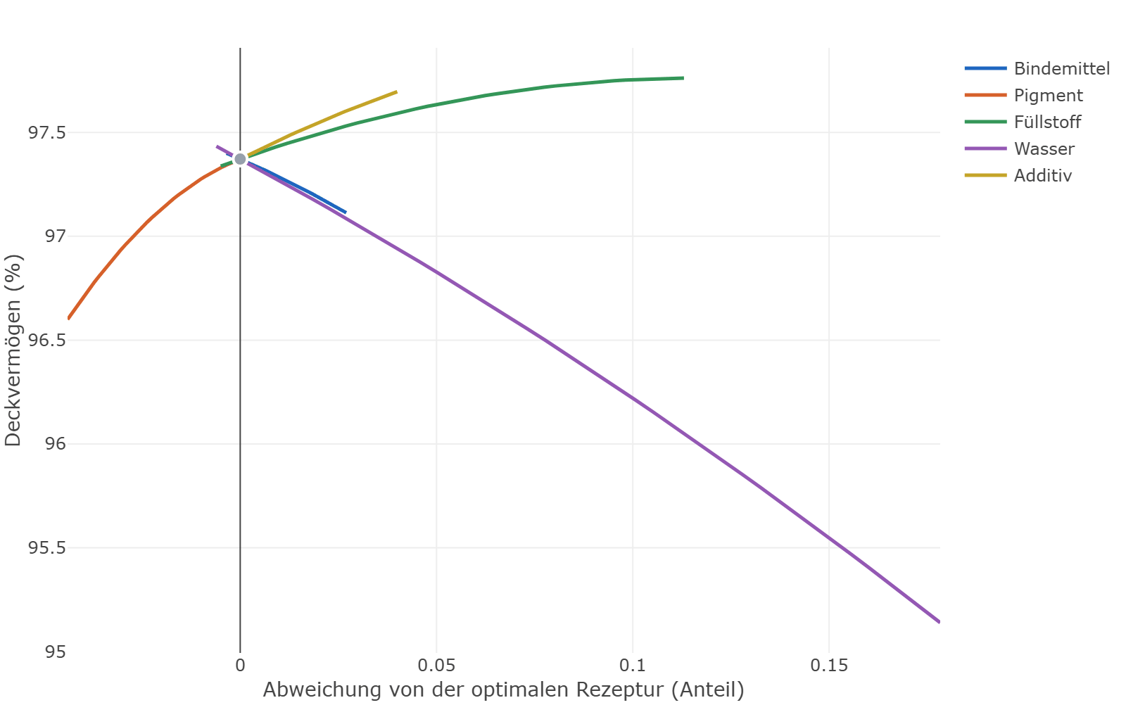
In a mixture there is no “change this component and hold everything else”. What one looks at instead: start at a reference recipe, move one component through its allowed range and let the others give way in the same proportion to one another. The table shows the change of each response along that path, starting from the centroid of the region.
| Component | Viscosity [KU] | Hiding power [%] | Wet scrub loss [µm] |
|---|---|---|---|
| Binder | 2.31 | −1.57 | −16.9 |
| Pigment | 20.0 | 3.09 | 3.24 |
| Filler | 36.7 | 0.930 | 10.7 |
| Water | −112 | −2.83 | 5.96 |
| Additive | 45.2 | 0.184 | −1.17 |
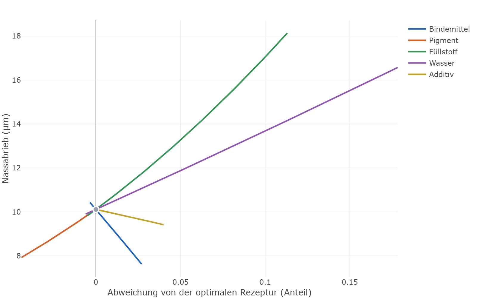
The roles are clearly divided. The viscosity depends on the water (−112 KU across its range) and on the additive, which moves 45 KU despite its small amount. The hiding power depends on the pigment, the wet scrub loss on the binder. The trace plots show the same as curves, here starting from the optimal recipe:
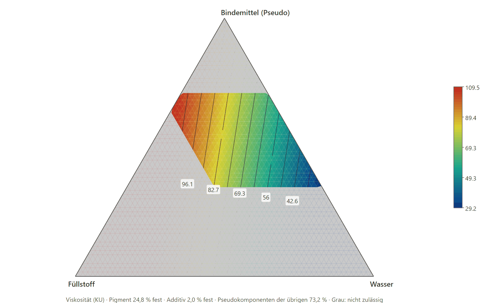
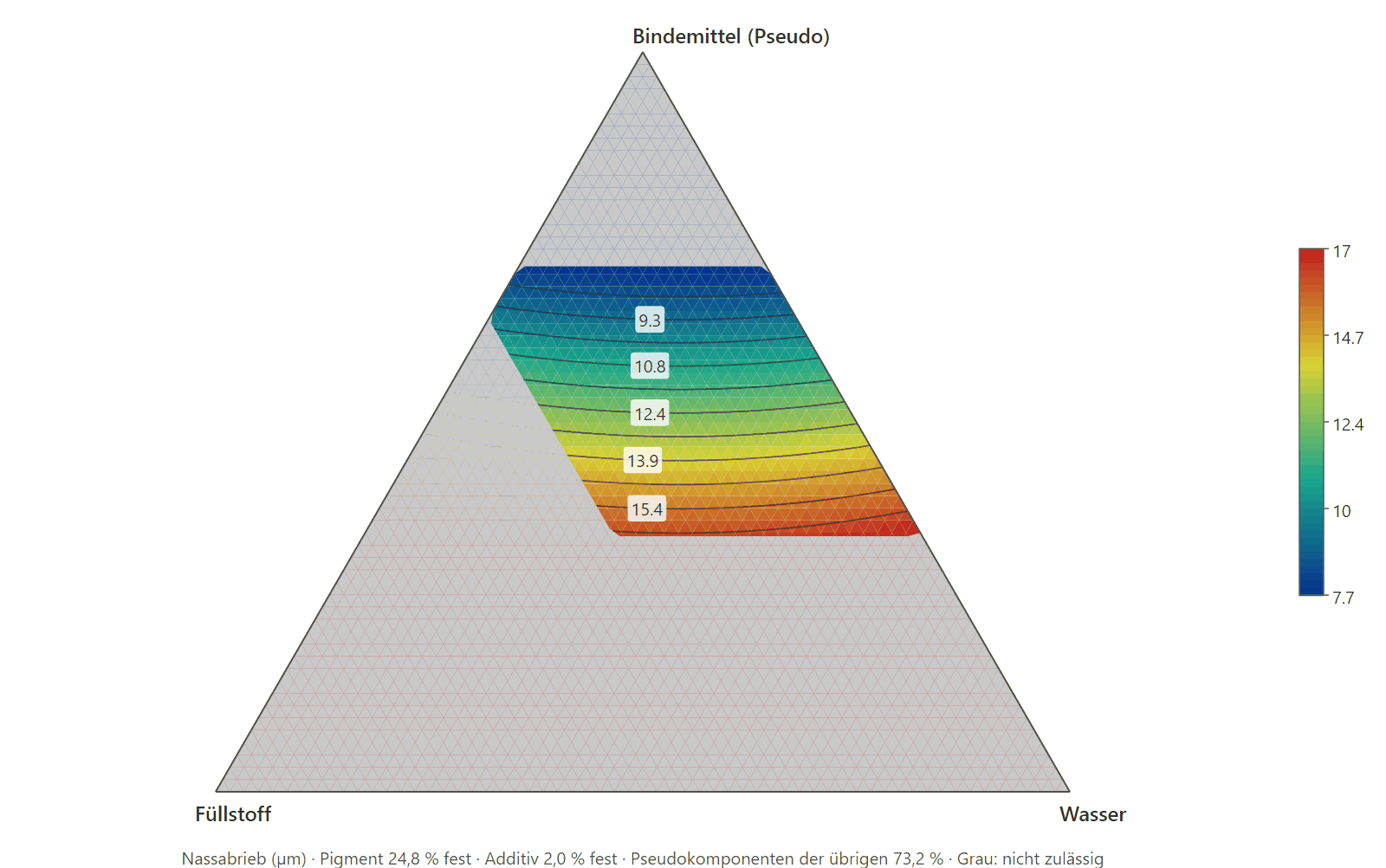
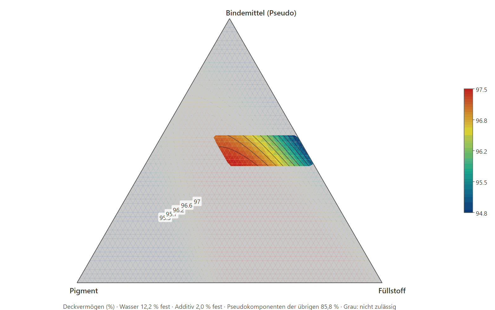
For surface pictures a mixture needs the triangle. Five components do not fit into it, so two are held — here at the values of the optimal recipe — and three share the rest among themselves. Grey is what the bounds and the two linking constraints exclude.
Step 6 / Optimisation
The best feasible recipe
As in the other examples, desirability combines the three goals into one number. The difference: the search is not in a cube but in the body with 28 vertices — every recipe examined must keep all bounds and both linking constraints and add up to 100%.
| Component | Share [%] | Allowed [%] |
|---|---|---|
| Binder | 47.3 | 30 … 50 |
| Pigment | 24.8 | 15 … 25 |
| Filler | 13.7 | 5 … 25 |
| Water | 12.2 | 10 … 30 |
| Additive | 2.0 | 2 … 6 |
| Pigment + filler | 38.5 | ≤ 40 |
| Binder : pigment | 1.90 | ≥ 1.6 |
| Response | Goal | Prediction | 95% prediction interval | Desirability d | True value |
|---|---|---|---|---|---|
| Viscosity [KU] | target 100 (90.0 … 110) | 100.0 | 94.0 … 106.0 | 1.000 | 100.2 |
| Hiding power [%] | maximise, at least 96.0 | 97.37 | 96.64 … 98.11 | 0.686 | 97.60 |
| Wet scrub loss [µm] | minimise, at most 20.0 | 10.1 | 7.3 … 12.9 | 0.824 | 8.6 |
| Overall desirability D | 0.827 |
The overall desirability is 0.83. The viscosity hits its target exactly. The recipe uses the region to the full: additive at its lower bound, pigment just below its upper bound, the solids sum at 38.5% close to the 40% allowed. The ratio of binder to pigment, at 1.90, is well above the minimum — the large amount of binder lowers the wet scrub loss.
Step 7 / Confirmation
Three batches of the recommended recipe
| Response | 95% prediction interval | Confirmation 1 | Confirmation 2 | Confirmation 3 | Joint test p |
|---|---|---|---|---|---|
| Viscosity [KU] | 94.0 … 106.0 | 100.1 | 95.4 | 104.2 | 0.2298 |
| Hiding power [%] | 96.64 … 98.11 | 97.49 | 97.75 | 97.32 | 0.7265 |
| Wet scrub loss [µm] | 7.3 … 12.9 | 9.9 | 10.6 | 9.0 | 0.8383 |
Result: all nine measurements lie within the prediction interval. The recipe delivers 100 KU, a hiding power of a little over 97% and about 10 µm wet scrub loss — with 25 trial batches instead of a grid over five components.
Cross-check
What is really in the data
The measurements come from these three models. The letters stand for the deviation of the share from a reference recipe (binder 40%, pigment 20%, filler 15%, water 20%, additive 5%), written as a fraction: b for binder, p for pigment, f for filler, w for water, a for additive.
Viscosity = 100 + 40·b + 220·p + 180·f − 380·w + 1100·a − 3000·w·a + 1200·p·f (σ = 2.0)
Hiding power = 96.5 − 4·b + 30·p + 6·f − 8·w − 250·p² + 40·p·f (σ = 0.25)
Wet scrub loss = 14 − 60·b + 25·p + 45·f + 20·w + 300·f² + 150·b·f (σ = 1.0)
For the viscosity the analysis found exactly the two blending terms that exist: pigment × filler and water × additive. For the hiding power the truth lies in a square of the pigment — the saturation the trace plot shows. A Scheffé model knows no squares; because the shares add up to one, p² appears there as the blending terms of the pigment with all the other components. Exactly those four the analysis kept. For the wet scrub loss the decomposition is less clear-cut: two blending terms with the filler were found, which reproduce the true filler square and its interaction with the binder well within the region studied but are not the same terms.
What counts is the prediction. At the optimal recipe the true values are 100.2 KU, 97.60% and 8.6 µm — predicted were 100.0, 97.37 and 10.1. All three lie within the prediction interval; for the wet scrub loss reality is somewhat better than the prediction.
Project files
Run it yourself
The example ships with DoEStat: Help ▸ Open sample project ▸ Mixture ▸ “Five-component mixture with constraints: emulsion paint”, once with the data only and once with the finished analysis. The same files can be downloaded here.
- Project with the datalack-mischung-daten.doejson
- Project with the finished analysislack-mischung-auswertung.doejson
Back: response surface with three responses Next: from screening to a response surface
Try DoEStat for free
30 days, the full feature set, no payment details. We send the download link by e-mail, usually on the next business day.