Examples / 04

From screening to a response surface: a design grows into a shifted region

A screening rarely ends with the answer — usually with the next question. Here it shows that three of six factors matter, that the surfaces are curved and that the optimum lies on the edge of the region studied. Instead of starting over, the 19 runs already made are carried along: into a slightly shifted region of the three active factors, augmented by 15 new runs until they carry a response surface for five responses.

Campaign 1: 2⁶⁻² fractional factorial, 16 + 3 = 19 runs
Campaign 2: I-optimal augmentation, 12 + 3 = 15 runs
Factors: 6, of which 3 active
Responses: 5 tablet properties

The measurements are simulated. They come from five models we set ourselves, plus random scatter — which makes it possible to check at the end whether the analysis finds what is really in there. Every table and chart was computed and drawn by DoEStat.

Step 1 / The question

One tablet, five requirements

A tablet should be strong enough to survive packaging and transport but disintegrate fast enough to release its active ingredient — and it should leave the die without damage. Five properties are measured on every batch:

Breaking force — target 100 N, 80 to 120 N allowed
Friability — to be minimised, at most 1.0%
Disintegration time — to be minimised, at most 15 min
Dissolution after 30 minutes — to be maximised, at least 85%
Ejection force — to be minimised, at most 350 N

Six quantities of formulation and press are candidate settings:

Factor	Unit	low (−1)	centre (0)	high (+1)
Compression force	kN	8.0	11.0	14.0
Turret speed	1/min	20	30	40
Lubricant	%	0.50	1.00	1.50
Blending time	min	2	6	10
Disintegrant	%	2.00	3.50	5.00
Granule moisture	%	1.5	2.5	3.5

Step 2 / Screening

Campaign 1: six factors in 19 runs

For six factors a regular fractional factorial is enough: 2⁶⁻², a quarter of the 64 combinations, resolution IV — main effects are clear of two-factor interactions. Three centre runs are added. The power for an effect of two standard deviations is 96%.

Run	Compression force [kN]	Turret speed [1/min]	Lubricant [%]	Blending time [min]	Disintegrant [%]	Granule moisture [%]	Breaking force [N]	Friability [%]	Disintegration time [min]	Dissolution [%]	Ejection force [N]
1	11.0	30	1.00	6	3.50	2.5	97	0.57	9.6	83.9	299
2	14.0	40	0.50	2	2.00	3.5	130	0.38	16.6	71.2	460
3	8.0	20	0.50	10	2.00	3.5	74	0.72	8.2	84.4	339
4	14.0	20	1.50	2	2.00	3.5	108	0.51	18.8	62.2	286
5	8.0	40	0.50	10	5.00	1.5	69	0.79	3.3	97.1	357
6	14.0	40	1.50	10	5.00	3.5	98	0.59	11.7	80.6	320
7	14.0	20	0.50	10	5.00	3.5	125	0.41	8.4	89.0	463
8	14.0	20	1.50	10	2.00	1.5	100	0.52	19.4	65.3	289
9	8.0	40	1.50	10	2.00	3.5	64	1.01	11.9	77.9	249
10	8.0	20	0.50	2	2.00	1.5	76	0.85	8.3	86.9	342
11	14.0	20	0.50	2	5.00	1.5	128	0.28	6.7	92.7	464
12	8.0	20	1.50	2	5.00	3.5	60	1.08	6.9	87.7	228
13	11.0	30	1.00	6	3.50	2.5	98	0.62	9.3	89.1	292
14	8.0	20	1.50	10	5.00	1.5	56	1.02	6.5	88.3	227
15	14.0	40	1.50	2	5.00	1.5	102	0.59	10.7	82.2	309
16	14.0	40	0.50	10	2.00	1.5	125	0.45	16.1	72.6	465
17	8.0	40	0.50	2	5.00	3.5	78	0.86	3.0	96.9	367
18	11.0	30	1.00	6	3.50	2.5	98	0.63	9.9	85.7	316
19	8.0	40	1.50	2	2.00	1.5	71	1.03	11.5	78.3	223

The analysis of the main effects for all five responses fits into one table. Each number is the effect of the factor from its low to its high level; highlighted is what is significant (p < 0.05).

Factor	Breaking force [N]	Friability [%]	Disintegration time [min]	Dissolution [%]	Ejection force [N]
Compression force	46.0	−0.454	6.10	−10.2	90.5
Turret speed	1.25	0.0388	0.200	0.0375	14.0
Lubricant	−18.2	0.201	3.35	−8.54	−141
Blending time	−5.25	−0.00875	0.375	−0.363	3.75
Disintegrant	−4.00	0.0187	−6.70	14.5	10.3
Granule moisture	1.25	0.00375	0.375	−1.69	4.50
Residual s	5.27	0.0667	1.11	3.21	21.4
Lack of fit p	0.0099	0.1792	0.0594	0.4494	0.2480

Pareto chart of the effects on breaking force: compression force and lubricant exceed the significance limit, the four other factors stay below it. — **Pareto: breaking force**Compression force and lubricant — nothing else.

Pareto chart of the effects on dissolution: disintegrant, compression force and lubricant exceed the significance limit, the three other factors stay below it. — **Pareto: dissolution**Here the disintegrant leads, ahead of compression force and lubricant.

Half-normal plot of the effects on disintegration time: three points – disintegrant, compression force, lubricant – lie far to the right beyond the limits, three lie close to zero on the line. — **Half-normal plot: disintegration time**Three effects stand out, three lie on the noise line.

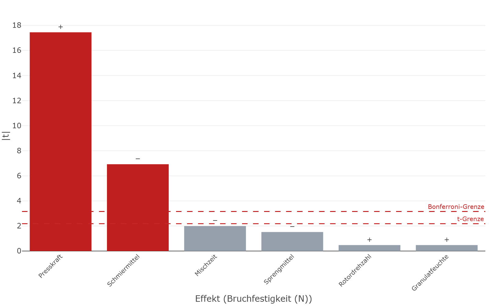
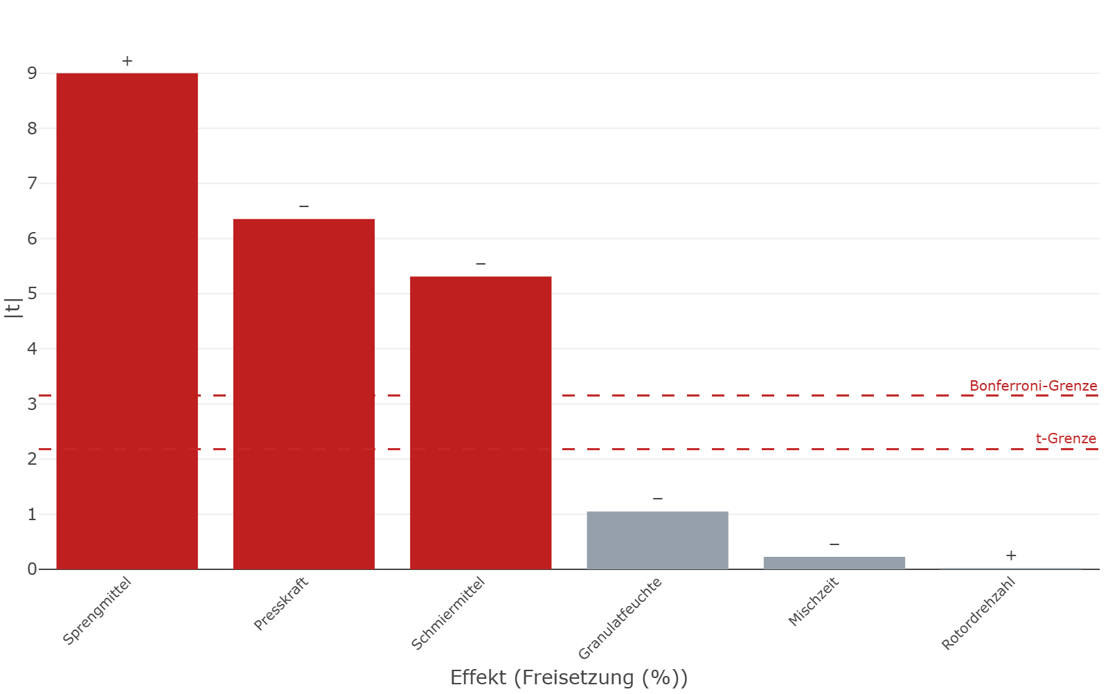
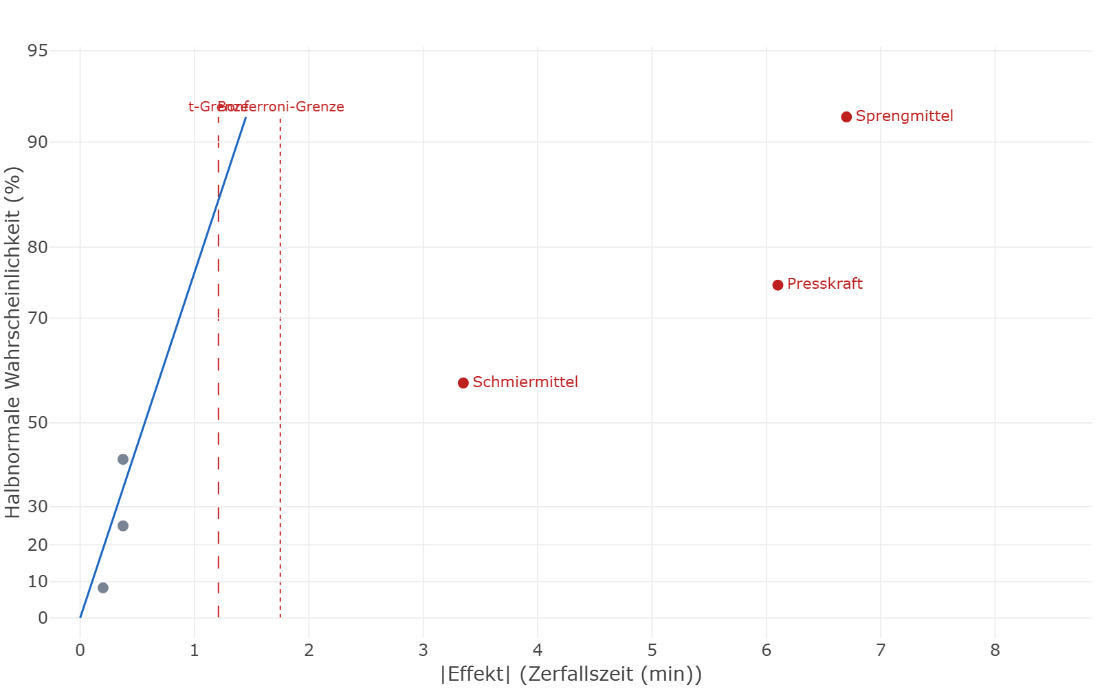
Finding 1: compression force and lubricant act on all five responses, the disintegrant on disintegration time and dissolution. Turret speed, blending time and granule moisture show no significant effect in any of the 15 tests. Three factors remain.

Step 3 / Findings

Why the screening is not the end

With the three active factors one can already optimise. Through desirability, the screening models (main effects and the interactions that prove significant) lead to this setting:

Quantity	Value in the screening region	Desirability d
Compression force [kN]	11.19
Lubricant [%]	1.051
Disintegrant [%]	5.000	on the boundary
Breaking force [N]	93.0	0.650
Friability [%]	0.675	0.541
Disintegration time [min]	7.32	0.768
Dissolution [%]	89.33	0.433
Ejection force [N]	327.0	0.230
Overall desirability D		0.493

Two things speak against stopping here.

The optimum lies on the edge. The disintegrant sits at its upper limit of 5%. A model made of straight lines always says “further in this direction” at an edge — whether there is more to gain beyond it or the effect has long flattened out, it cannot know.

The surfaces are curved. The three centre runs lie beside what the models predict for the centre: for the ejection force 302 N measured against 331 N predicted (lack of fit p < 0.001), for the dissolution 86.2% against 82.7% (p = 0.044). A two-level design can detect this curvature but cannot assign it to a factor.

Finding 2: what is needed is a quadratic model for three factors — and a region that reaches beyond 5% for the disintegrant.

Step 4 / Augmenting

Campaign 2: shift the region, augment the design

The three inactive factors are fixed — at values that suit production:

Factor	In the screening	Held in the second campaign at
Turret speed	20 … 40 1/min	40 1/min
Blending time	2 … 10 min	5 min
Granule moisture	1.5 … 3.5 %	2.5 %

For the three active ones the region is redrawn. For the disintegrant it moves up, so that the previous upper limit lies in the middle; for the lubricant the lower edge, where the ejection force was too high, is dropped; for the compression force it becomes narrower around the range in which the breaking force meets its window.

Factor	Unit	Screening	Second campaign	Old levels on the new scale (coded)
Compression force	kN	8.0 … 14.0	9.0 … 13.0	−1.50 … 1.50
Lubricant	%	0.50 … 1.50	0.75 … 1.50	−1.67 … 1.00
Disintegrant	%	2.00 … 5.00	3.50 … 6.50	−2.00 … 0.00

In DoEStat this is one function: change the factor range and augment the design for a target model. The 19 existing runs are kept with their measurements and re-coded to the new scale — the last column shows where the old levels lie there. 16 of the 19 runs lie outside the new cube; DoEStat points out that the model computes outside the new region there. They still support the surface from outside. To these DoEStat adds, I-optimally, twelve new points in the new region that together with the old ones carry the quadratic model best, and three new centre runs.

Run	Campaign	Compression force [kN]	Lubricant [%]	Disintegrant [%]	Breaking force [N]	Friability [%]	Disintegration time [min]	Dissolution [%]	Ejection force [N]
1	1	11.0	1.00	3.50	97	0.57	9.6	83.9	299
2	1	14.0	0.50	2.00	130	0.38	16.6	71.2	460
3	1	8.0	0.50	2.00	74	0.72	8.2	84.4	339
4	1	14.0	1.50	2.00	108	0.51	18.8	62.2	286
5	1	8.0	0.50	5.00	69	0.79	3.3	97.1	357
6	1	14.0	1.50	5.00	98	0.59	11.7	80.6	320
7	1	14.0	0.50	5.00	125	0.41	8.4	89.0	463
8	1	14.0	1.50	2.00	100	0.52	19.4	65.3	289
9	1	8.0	1.50	2.00	64	1.01	11.9	77.9	249
10	1	8.0	0.50	2.00	76	0.85	8.3	86.9	342
11	1	14.0	0.50	5.00	128	0.28	6.7	92.7	464
12	1	8.0	1.50	5.00	60	1.08	6.9	87.7	228
13	1	11.0	1.00	3.50	98	0.62	9.3	89.1	292
14	1	8.0	1.50	5.00	56	1.02	6.5	88.3	227
15	1	14.0	1.50	5.00	102	0.59	10.7	82.2	309
16	1	14.0	0.50	2.00	125	0.45	16.1	72.6	465
17	1	8.0	0.50	5.00	78	0.86	3.0	96.9	367
18	1	11.0	1.00	3.50	98	0.63	9.9	85.7	316
19	1	8.0	1.50	2.00	71	1.03	11.5	78.3	223
20	2	13.0	1.05	6.50	99	0.65	7.9	85.3	341
21	2	9.0	1.05	6.50	76	0.93	7.0	91.0	264
22	2	13.0	1.05	4.40	107	0.61	9.3	84.5	328
23	2	11.0	1.50	4.10	92	0.76	10.0	81.2	265
24	2	11.0	1.50	6.50	84	0.75	9.0	85.0	287
25	2	11.0	1.05	4.10	94	0.58	8.9	86.2	310
26	2	9.0	0.98	6.50	77	0.87	5.9	88.0	306
27	2	11.0	1.50	6.50	83	0.84	8.4	81.0	279
28	2	11.0	1.50	4.10	83	0.70	10.1	82.5	281
29	2	11.8	0.75	6.50	100	0.59	6.6	88.4	373
30	2	11.0	0.98	4.10	101	0.73	8.2	88.2	322
31	2	11.0	1.05	4.10	95	0.54	8.2	89.1	303
32	2	11.0	1.13	5.00	91	0.76	8.0	87.0	297
33	2	11.0	1.13	5.00	90	0.69	6.9	89.5	299
34	2	11.0	1.13	5.00	88	0.73	8.3	89.4	290

The new runs are highlighted in the table. What the augmentation achieves is shown by the design evaluation: with the 19 old runs alone the quadratic model cannot be estimated. With all 34 it can, with variance inflation below 4 and a power of 86 to 100% per term for an effect of one standard deviation:

Term	VIF	Power at 1 σ
Compression force	1.65	99.7
Lubricant	2.00	98.1
Disintegrant	2.46	95.2
Compression force × Lubricant	1.07	100.0
Compression force × Disintegrant	1.59	100.0
Lubricant × Disintegrant	1.79	100.0
Compression force²	2.67	95.0
Lubricant²	3.65	85.9
Disintegrant²	2.65	100.0

A side effect of dropping factors: because the three removed factors have no effect, the 16 corners of the screening are, in the space of the three remaining ones, eight corners each run twice. Together with the centre runs of both campaigns that gives 15 degrees of freedom for pure error — a reliable estimate of scatter that cost no additional run.

Step 5 / Response surface

Five models from 34 runs

Every response gets its own model: reduced backwards from the full quadratic model (p-value, α = 0.05, hierarchy kept).

Response	Terms in the model	R²	Adj. R²	Pred. R²	Residual s	Lack of fit p	Campaign share of variance
Breaking force [N]	5	0.9729	0.9681	0.9567	3.33	0.6112	0.0%
Friability [%]	4	0.9169	0.9054	0.8862	0.0594	0.0895	27.3%
Disintegration time [min]	5	0.9879	0.9857	0.9819	0.442	0.9637	0.0%
Dissolution [%]	5	0.9641	0.9576	0.9476	1.57	0.8898	0.0%
Ejection force [N]	5	0.9806	0.9771	0.9702	9.76	0.1155	5.0%

Term (coded)	Breaking force [N]	Friability [%]	Disintegration time [min]	Dissolution [%]	Ejection force [N]
Intercept	92.1	0.689	7.63	88.3	296
Compression force	14.5	−0.149	1.42	−2.37	28.4
Lubricant	−6.77	0.0750	1.26	−3.30	−40.4
Disintegrant	−2.46	0.0303	−1.20	1.11	5.92
Compression force × Lubricant	−1.69	·	·	·	−5.26
Compression force × Disintegrant	·	·	−0.585	1.12	·
Lubricant × Disintegrant	·	·	·	·	·
Compression force²	−2.35	0.0286	·	·	·
Lubricant²	·	·	·	·	17.8
Disintegrant²	·	·	1.06	−3.07	·

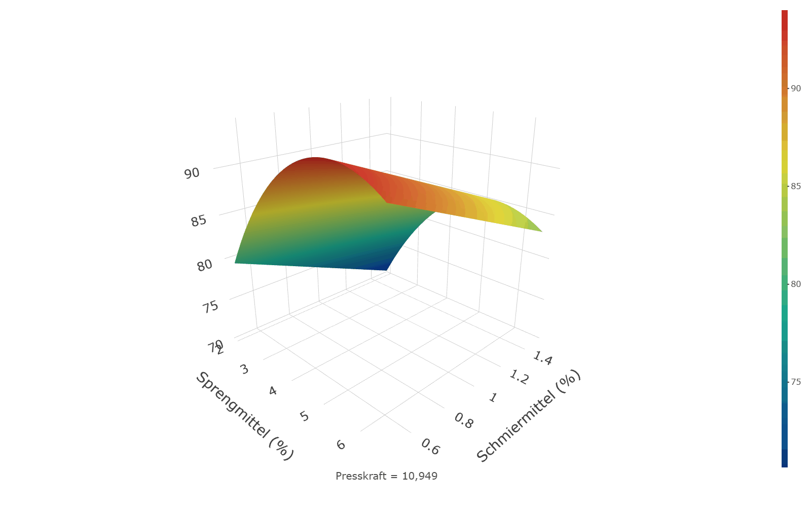
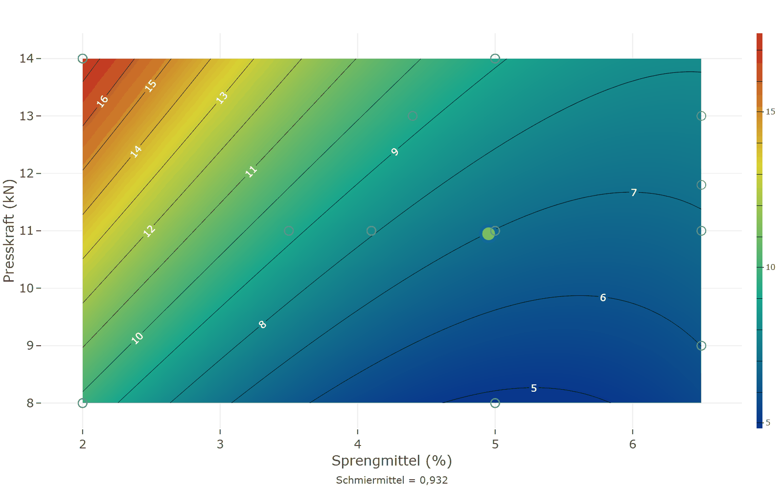
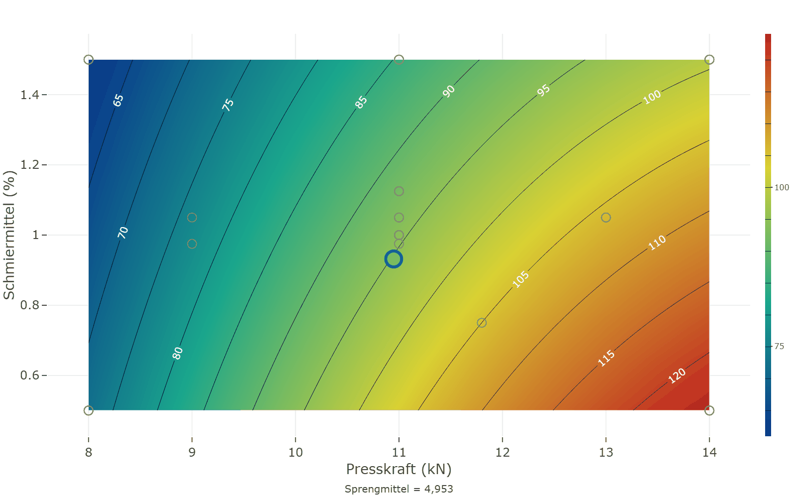
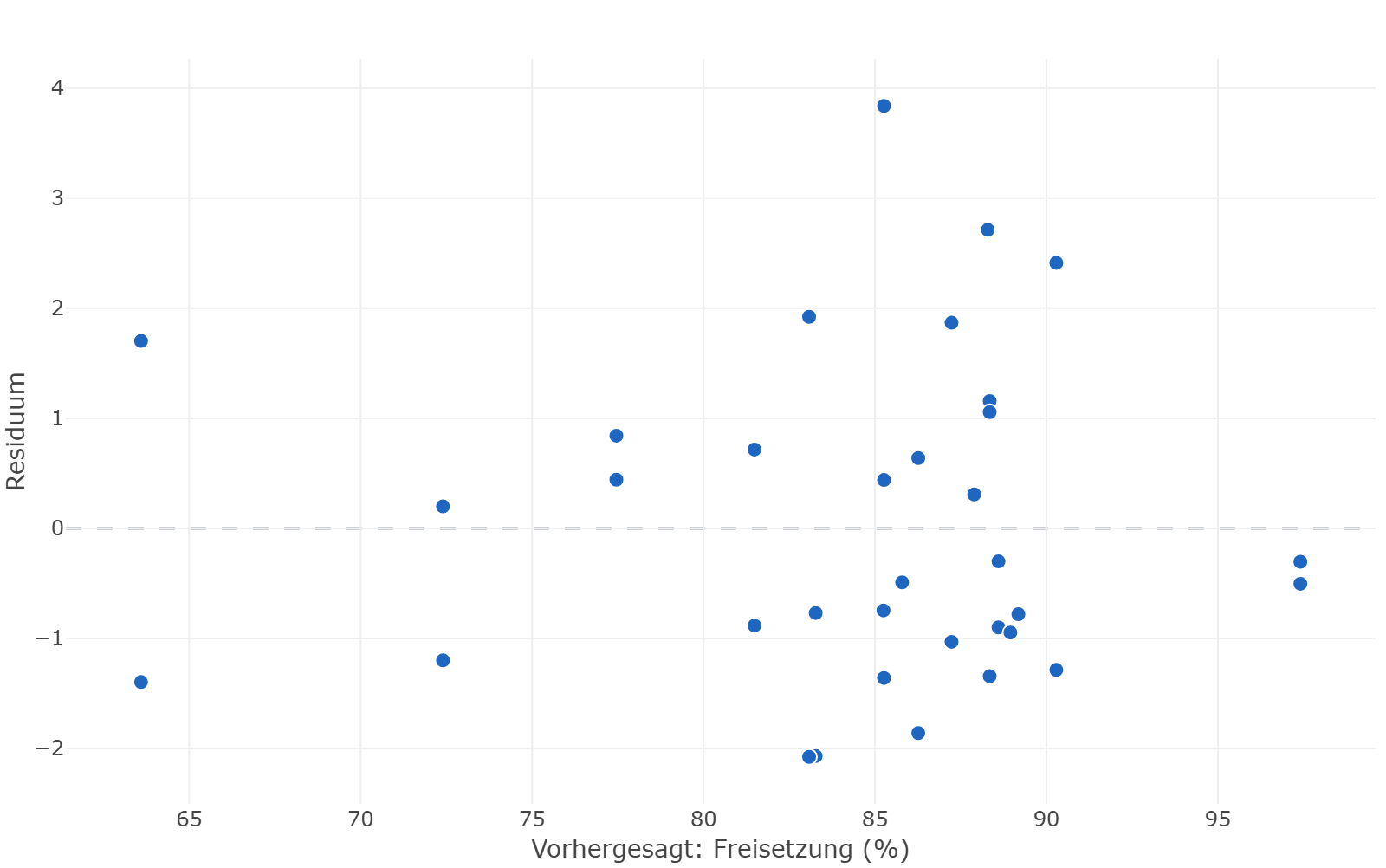
The coefficients are in the coded units of the new region. The curvature the screening could only detect now has a name: disintegrant² for disintegration time and dissolution, lubricant² for the ejection force, compression force² for breaking force and friability. The lack of fit is no longer significant for any response.

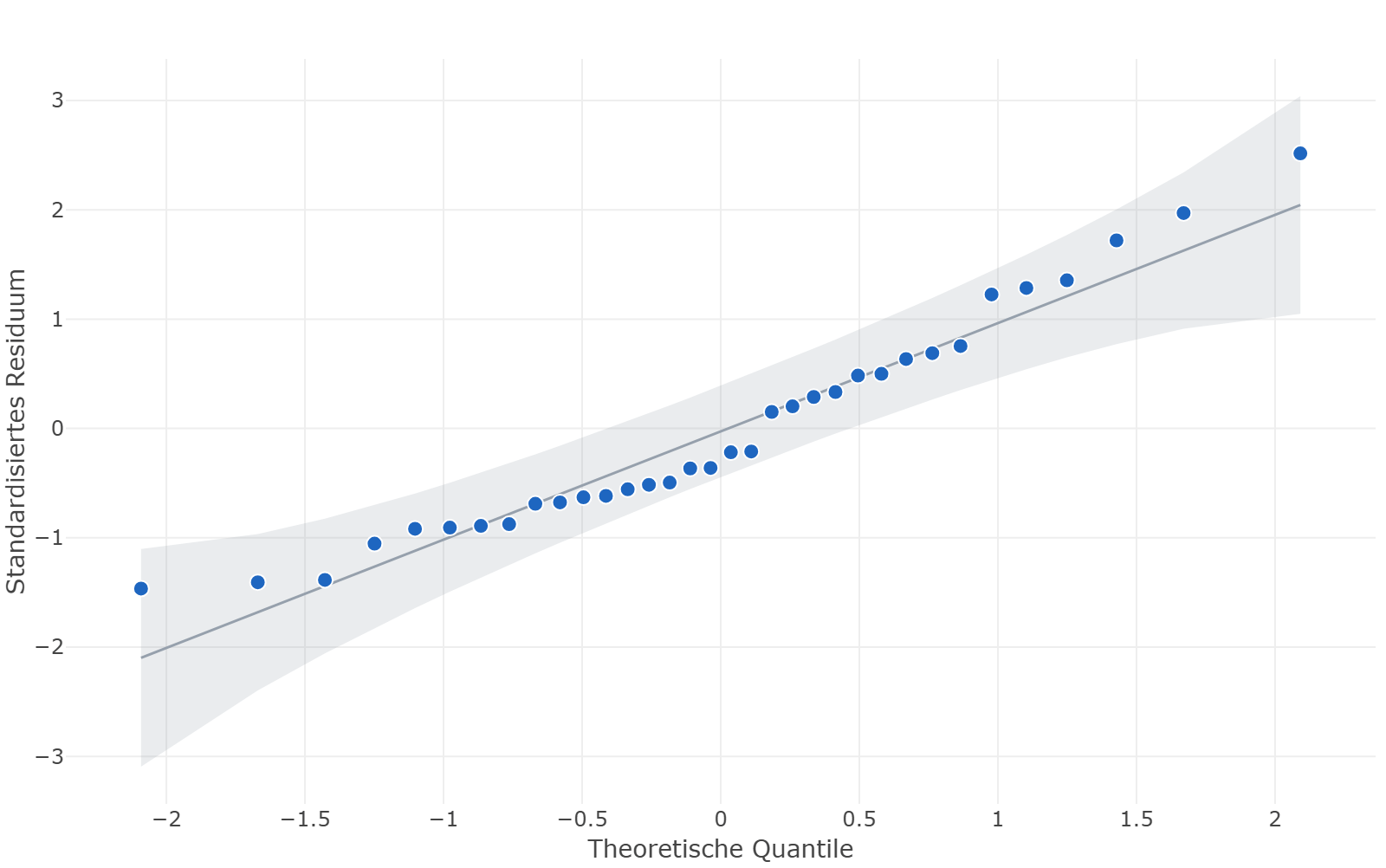
Do the campaigns differ? Weeks may lie between two series of runs, a new raw-material lot, a different operator. DoEStat carries the campaign as a block and can estimate it as a random effect. The last column shows the campaign’s share of the residual variation: zero for three responses, 5% for the ejection force, 27% of an already small variation for the friability. The campaigns fit together.

Analysis of variance of the dissolution

Source	Sum of squares	df	Mean square	F	p
Model	1861	5	372.2	150.22	< 0.0001
Compression force	142.5	1	142.5	57.50	< 0.0001
Lubricant	381.0	1	381.0	153.75	< 0.0001
Disintegrant	17.64	1	17.64	7.12	0.0125
Compression force × Disintegrant	60.14	1	60.14	24.27	< 0.0001
Disintegrant²	323.7	1	323.7	130.63	< 0.0001
Residual	69.38	28	2.478
Lack of fit	21.06	13	1.620	0.50	0.8898
Pure error	48.32	15	3.221
Total	1930	33

Contour plot of the dissolution over disintegrant from 2 to 6.5 per cent and lubricant from 0.5 to 1.5 per cent, with the runs of both campaigns: the dissolution rises with the disintegrant up to about 5.3 per cent and falls again after that; less lubricant raises it. The optimal setting is marked. — **Dissolution: disintegrant × lubricant**Old and new region on one map. The dissolution peaks at a little over 5% disintegrant — beyond the old upper limit it falls again.

Three-dimensional response surface of the dissolution over disintegrant and lubricant: a ridge that rises and falls again along the disintegrant. — **The same surface in 3D**A ridge: curved along the disintegrant, falling almost straight along the lubricant.

Contour plot of the disintegration time over disintegrant and compression force: the disintegration time falls with the disintegrant down to a flat valley and rises with the compression force. — **Disintegration time: disintegrant × compression force**Here too the effect of the disintegrant flattens out; more compression force prolongs disintegration.

Contour plot of the breaking force over compression force and lubricant: the strength rises with the compression force and falls with the lubricant. — **Breaking force: compression force × lubricant**Compression force hardens, lubricant softens — the line for 100 N runs diagonally through the region.

Residuals of the dissolution against predicted values: the points of both campaigns scatter evenly around the zero line. — **Residuals against prediction**Dissolution, both campaigns: no structure.

Normal quantile plot of the standardised residuals of the dissolution: the points follow the straight line. — **Normality of the residuals**The points follow the line.

Step 6 / Optimisation

One window for five requirements

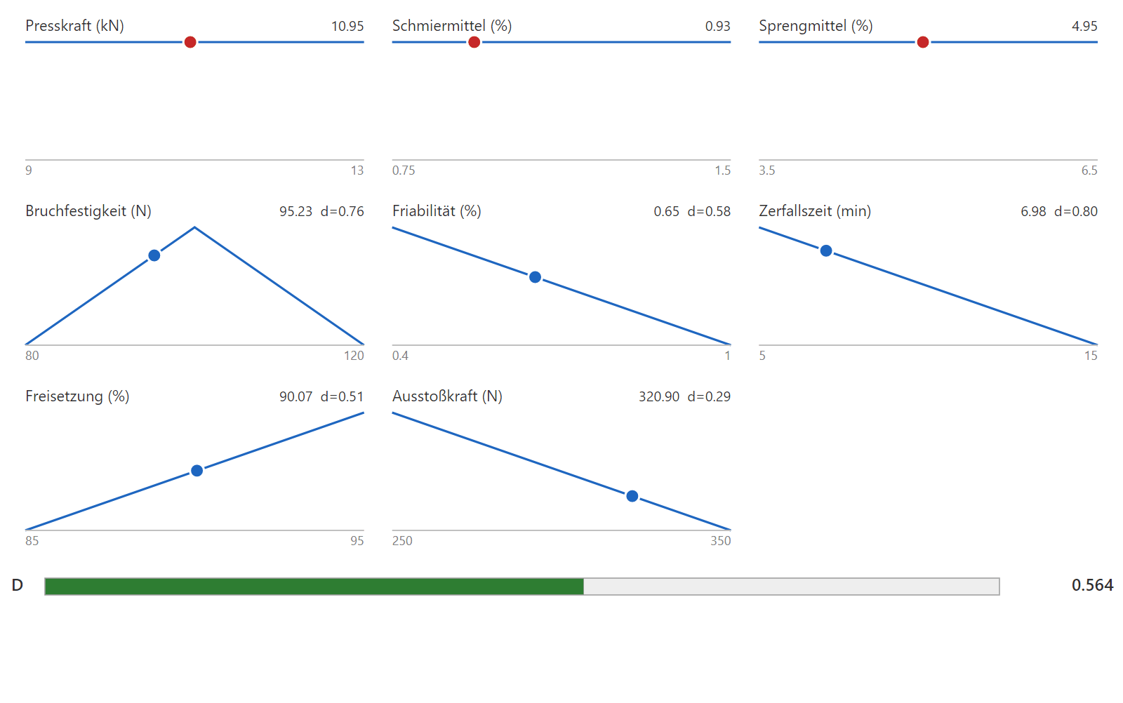
Desirability combines the five goals; the search is in the new region.

Factor	Setting	Unit	coded
Compression force	10.95	kN	−0.03
Lubricant	0.932	%	−0.52
Disintegrant	4.953	%	−0.03

Response	Goal	Prediction	95% prediction interval	Desirability d	True value
Breaking force [N]	target 100 (80.0 … 120)	95.2	88.2 … 102.3	0.762	93.1
Friability [%]	minimise, at most 1.00	0.653	0.527 … 0.779	0.578	0.649
Disintegration time [min]	minimise, at most 15.0	6.98	6.05 … 7.91	0.802	7.05
Dissolution [%]	maximise, at least 85.0	90.07	86.75 … 93.38	0.507	90.63
Ejection force [N]	minimise, at most 350	320.9	300.2 … 341.6	0.291	322.2
Overall desirability D				0.564

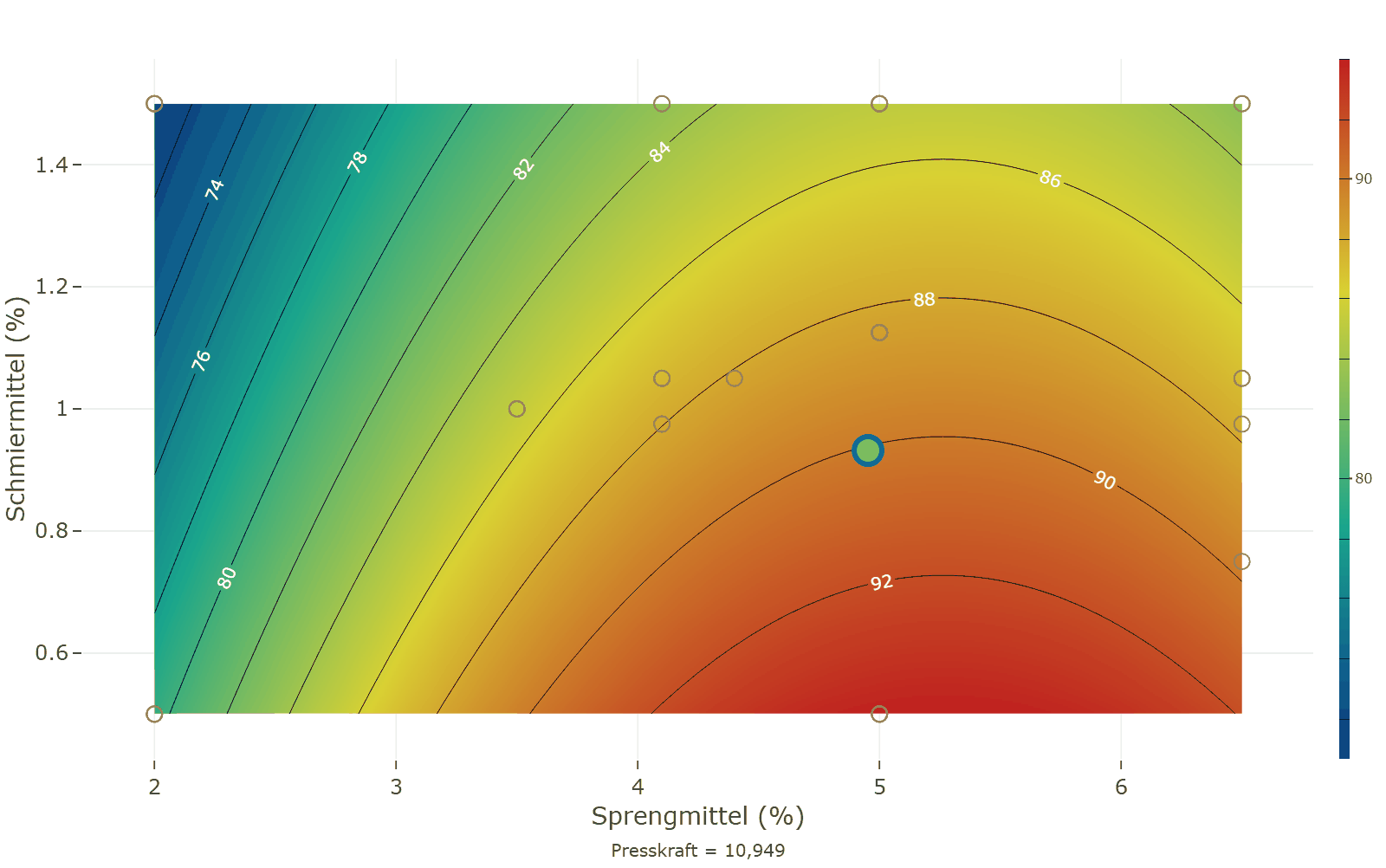
The optimum now lies in the interior: 4.95% disintegrant, 0.93% lubricant, 10.9 kN compression force. All five requirements are met, and the overall desirability is 0.56. The tightest is the ejection force: less lubricant helps dissolution, strength and disintegration but drives up the force at ejection — the compromise lies where the two balance.

Overlay plot over disintegrant and compression force: a large yellow feasible region, bounded at the top by ejection force equals 350, at the bottom by breaking force equals 80 and at the upper left by dissolution equals 85; a crosshair marks the optimal setting in the middle. — **Overlay: the feasible window**Yellow is where all five requirements are met. The setting lies in the middle of the window — clear of every border.

Ramps plot: at the top three sliders for the factors, below a ramp for each of the five responses with the predicted value as a point, at the bottom a bar for the overall desirability of 0.564. — **Ramps**Five responses at a glance: the breaking force close to its target, the ejection force furthest from its ideal.

All five responses in one picture

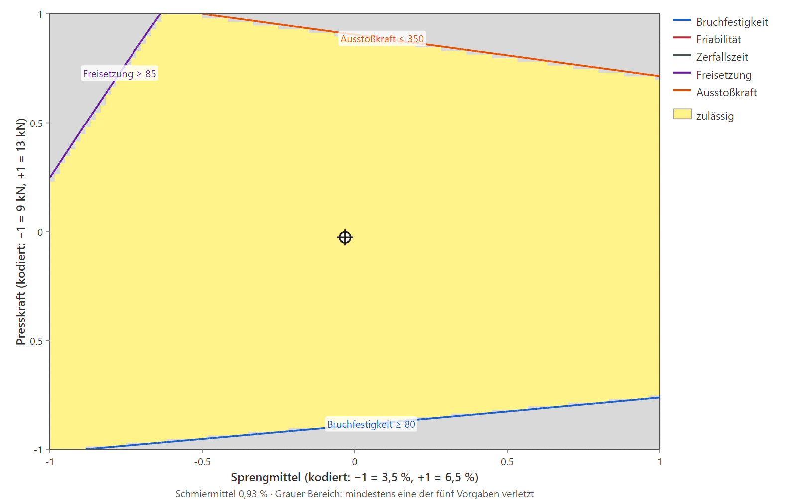
The overlaid view shows more than the limits: the contour lines of every response in its own colour, the limits as heavy lines — solid for a lower limit, dashed for an upper one — the sweet spot shaded and the optimum as a dot. Shown is the new region, one cut for each pair of factors.

Overlaid contour plot over disintegrant and lubricant with contour lines of five responses in five colours. The shaded region is bounded at the top by the heavy violet line dissolution equals 85 as an arc and at the bottom by the dashed orange line ejection force equals 350; the optimum lies at just under 5 per cent disintegrant and a little over 0.9 per cent lubricant. — **Disintegrant × lubricant**Two limits cut the window: dissolution at the top, ejection force at the bottom. The line for 90% dissolution shows the peak at a little over 5% disintegrant.

Overlaid contour plot over disintegrant and compression force with contour lines of five responses. The shaded region fills almost the whole picture; it is bounded at the upper left by the heavy violet line dissolution equals 85, at the top by the dashed orange line ejection force equals 350 and at the bottom by the heavy blue line breaking force equals 80. — **Disintegrant × compression force**Too much compression force drives the ejection force, too little costs breaking force; little disintegrant at high compression force costs dissolution.

Overlaid contour plot over compression force and lubricant with contour lines of five responses. The shaded region is bounded on the left by the heavy blue line breaking force equals 80, at the upper right by the heavy violet line dissolution equals 85 and at the lower right by the dashed orange line ejection force equals 350. — **Compression force × lubricant**Here three limits meet. The optimum lies on the line for 90% dissolution, between the lines for 300 and 350 N ejection force.

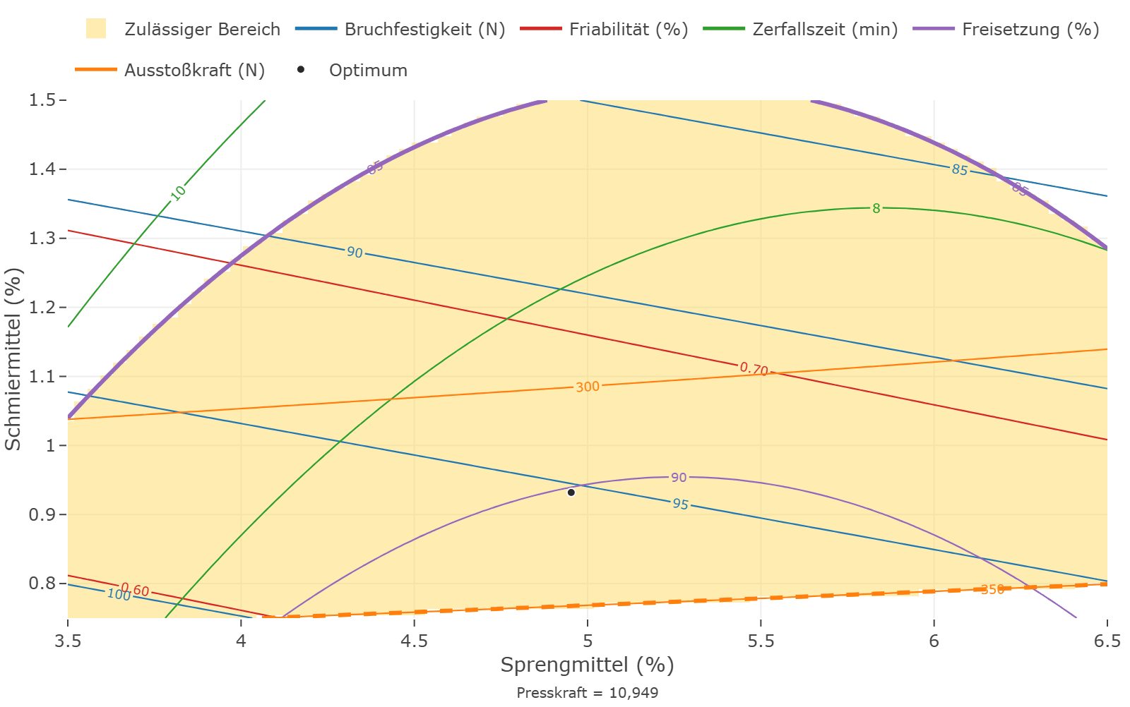
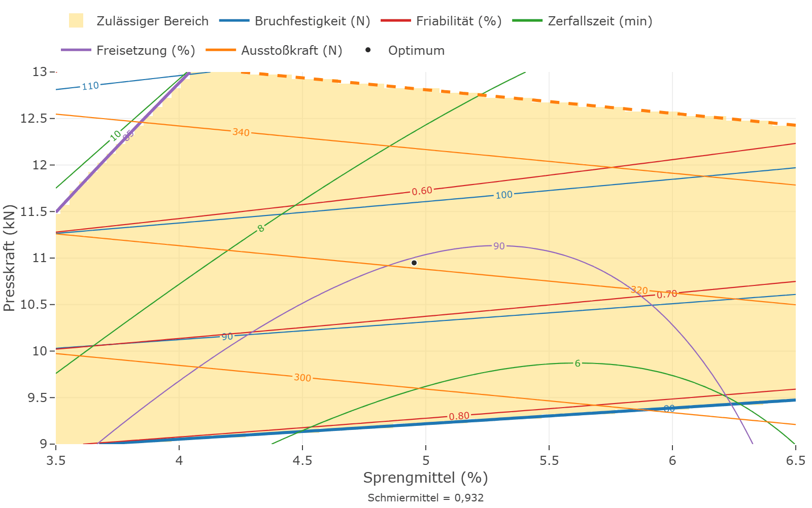
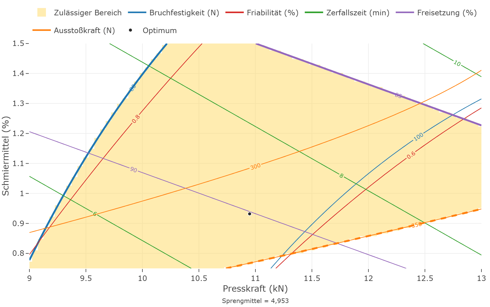
Three of the five requirements determine the window — dissolution, ejection force and breaking force. Friability and disintegration time keep their limits throughout the new region; their limit lines do not appear in the pictures at all. Anyone who wants to widen the latitude thus knows which three responses to work on.

Step 7 / Confirmation

Three batches at the recommended setting

Response	95% prediction interval	Confirmation 1	Confirmation 2	Confirmation 3	Joint test p
Breaking force [N]	88.2 … 102.3	98	94	89	0.2815
Friability [%]	0.527 … 0.779	0.64	0.62	0.63	0.9211
Disintegration time [min]	6.05 … 7.91	7.3	6.9	6.7	0.8224
Dissolution [%]	86.75 … 93.38	91.3	91.5	90.8	0.6699
Ejection force [N]	300.2 … 341.6	314	324	327	0.8200

Result: all 15 measurements lie within the prediction interval of their response, and no joint test responds.

Summing up

What the second step achieved

After both steps the disintegrant sits at about 5%. What has changed is what is known about it: after the screening that was an edge at which the model said “more”. After the augmentation it is an optimum — the map shows that the dissolution falls again beyond a little over 5%. Anyone who had followed the linear model and gone up to 6% would have used disintegrant and lost dissolution.

Lubricant and compression force have moved (from 1.05 to 0.93% and from 11.2 to 10.9 kN), and the overall desirability has risen from 0.49 to 0.56. Above all there are now models that describe curvature, with prediction intervals from 15 degrees of freedom of pure error — and an overlay that shows how much latitude the setting has.

The effort: 34 runs for six factors and five responses, of which not a single one was discarded. A fresh central composite design for three factors would have needed 20 runs on its own, in addition to the 19 of the screening.

Against the truth: the column “True value” in the optimisation table shows what the simulated models actually deliver at the recommended setting. All five true values lie within the prediction interval; the largest deviation is in the breaking force, at 2 N. The true models also contain tiny effects of the three dropped factors (at most 3 N of ejection force, 1 N of breaking force) — too small to show up in the screening, and too small to matter.

Project files

Run it yourself

The example ships with DoEStat as two projects — one per campaign: Help ▸ Open sample project ▸ Screening ▸ “Screening, first campaign: tabletting” and Response surface (RSM) ▸ “Augmented to a response surface: tabletting, both campaigns”, each with the data only and with the finished analysis. The same files can be downloaded here.

Campaign 1: project with the datatablette-screening-daten.doejson
Campaign 1: project with the finished analysistablette-screening-auswertung.doejson
Campaigns 1 + 2: project with the datatablette-wirkflaeche-daten.doejson
Campaigns 1 + 2: project with the finished analysistablette-wirkflaeche-auswertung.doejson

Back: mixture with constraints All examples

Try DoEStat for free

30 days, the full feature set, no payment details. We send the download link by e-mail, usually on the next business day.

Request the trial